Project 1 - Parsing NASA thermodynamic data
- To Write a function that extracts the 14 co-efficients and to calculates the enthalpy, entropy and specific heats for all the species in the data file.
- To find the molecular weight of each species
- To Plot the Cp, Enthalpy and Entropy for the local temperature range
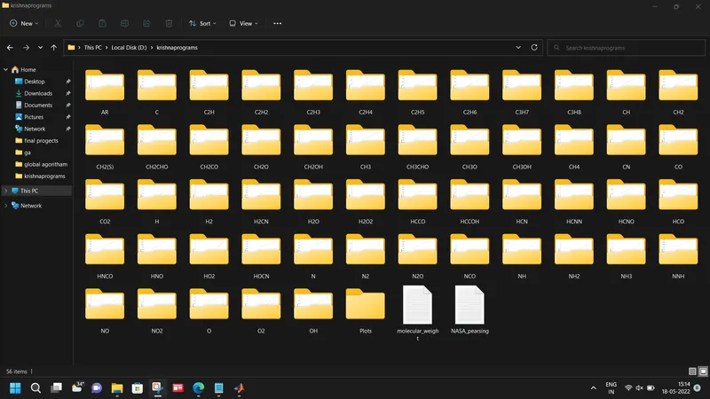
- To Save the plots as images with appropriate names and dump them in separate folders for each species with suitable name.
- The main program is to generate Cp, H and S plots.
OBJECTIVE:
NASA came up with a thermodynamic data which is used to evaluate the properties such as Specific heat (c_p),Enthalpy(H),Entropy(S).
And Pearsing a file means Reading data from a specific file and bilding an in memory model of semantic cuntent of the data.
Given Equations:
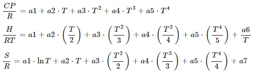
Where :
- CP = specific heat
- R = Universal gas constant
- S = entropy
- H = enthalpy
THEARY: File parsing is basically refers to how information basically read from text file or any type of file
By using file parsing we can able to read the data from external files or external databases
and we can include that data in the calculation.
In big data processing there is usually an interface between the program and large amount of data
weather the data is stored in a file or it comes from a server whatever it is ability to read the file and
take the data from it, and ability to store the useful information from the file.
DEFINITIONS:
- Specific Heat: Specific heat is a ratio of the quantity of heat required to raise the temperature of a body one digree to that required to raise the temperature of an equal mass of water one degree. The Si unit of specific heat is j/kg-k
- Enthalpy: The Enthalpy of a thermodynamic system is defined as the sum of internal energy and the work required to achieve its pressure and volume. The Si unit of specific Enthalpy is kj/kg.
- Entropy: Entropy is a measure of digree of disorderness of the system. the si unit of Entropy is j/k.
CODE LOGIC
-
To start off in almost all codes we use clear all, close all and clc.
-
Now we have to open the file from which we have to take and "Parsing" the data. by using fopen command
- To save the local temperature files using strfind command to Find the index of each letter, sequence of letters having throughout the length,
- Then converting a cell array of character vectors to a numeric array of the same size by using str2double
- Range of temperature for which the cp, h and s are calculated
- And extracting the global temperature local temperature & extracting the co-efficients
- Creates a new folder for saving plots use command mkdir('Plots').
- Specifying the location where the plots have to be saved cd('D' or 'C' or 'E' Drives:\give the name of the folder).
- Creating folder within the main folder with the name of each compound use the code mkdir(species_name).
- To save the images of the last compound in its own directory use command cd(species_name).
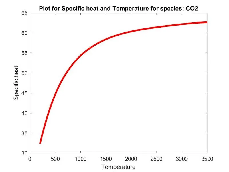
- Give the figure number & plot the temperature t, Specific heat (c-p) and give the line width and collor of the line And labling the parts also the title of the plot
- To redirect MATLAB to a new directory wher the function is saved.
- Previously the directory of matlab had been changed to new folder named plots .
- In "plots" Al the plots had been saved with respect to each compound.
- To call the function give the same name which you have given in the function program.
- To remove unwanted warning mesages in the command window use warning('off','all').
MAIN CODE
clear all
close all
clc

%opening the file and extracting the data
fid=fopen('THERMO.dat','r');
% str=textscan(fid,'%s','HeaderLines',0,'delimiter','\r\n');
class(fid)

for j=1:5
   b=fgetl(fid);
end

% 217-5=212, 212/4=53;
 for i=1:53

        one=fgetl(fid);
        A=strsplit(one,' ');
        species_name=(A{1});
        class(species_name);
%  To save local temperature files
        T=strfind(one,'G');
        t_one=str2double(one(T+3:T+7));
        t_two=str2double(one(T+12:T+20));
        t_three=str2double(one(T+22:T+30));

        t_array=linspace(t_one,t_two,2000);

        two=fgetl(fid);
        c_1=str2double(two(1:15));
        c_2=str2double(two(16:30));
        c_3=str2double(two(31:45));
        c_4=str2double(two(46:60));
        c_5=str2double(two(61:75));

        three=fgetl(fid);
        c_6=str2double(three(1:15));
        c_7=str2double(three(16:30));
        c_8=str2double(three(31:45));
        c_9=str2double(three(46:60));
        c_10=str2double(three(61:75));

        four=fgetl(fid);
        c_11=str2double(four(1:15));
        c_12=str2double(four(16:30));
        c_13=str2double(four(31:45));
        c_14=str2double(four(46:60));

        R=8.314462618;

        for k=1:length(t_array)
            if t_array(k)>t_three
                cp(k)=R.*(c_1+c_2.*t_array(k)+c_3.*t_array(k).^2+c_4.*t_array(k).^3+c_5.*t_array(k).^4);
                h(k)=R.*t_array(k)*(c_1+c_2.*(t_array(k))./2+c_3.*(t_array(k))./3+c_4.*(t_array(k))./4+c_5.*(t_array(k))./5+c_6./t_array(k));
                s(k)=R*(c_1.*log(t_array(k))+c_2.*t_array(k)+c_3.*(t_array(k)^2)./2+c_4.*(t_array(k)^3)./3+c_5.*(t_array(k).^4)./4+c_7);

            else
                cp(k)=R.*(c_8+c_9.*t_array(k)+c_10.*t_array(k).^2+c_11.*t_array(k).^3+c_12.*t_array(k).^4);
                h(k)=R.*t_array(k).*(c_8+c_9.*(t_array(k))./2+c_10.*(t_array(k))./3+c_11.*(t_array(k))./4+c_12.*(t_array(k))./5+c_13./t_array(k));
                s(k)=R.*(c_8*log(t_array(k))+c_9.*t_array(k)+c_10.*(t_array(k).^2)/2+c_11.*(t_array(k).^3)/3+c_12.*(t_array(k).^4)./4+c_14);
            end
        end

        % Creates a new folder for saving plots
        mkdir('Plots')
        % Specifying the location where the plots have to be saved
        cd('D:\krishnaprograms')
        % Creating folder within the main folder with the name of each compound
        mkdir(species_name);
        % To save the images of the last compound in its own directory
        cd(species_name);

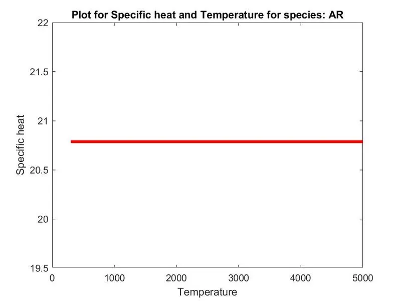
                figure(1)
                plot(t_array,cp,'linewidth',3,'color','r')
                xlabel('Temperature')
                ylabel('Specific heat')
                title(sprintf('Plot for Specific heat and Temperature for species: %s', species_name))
                saveas(figure(1),'Temperature Vs Specific heat.jpg')

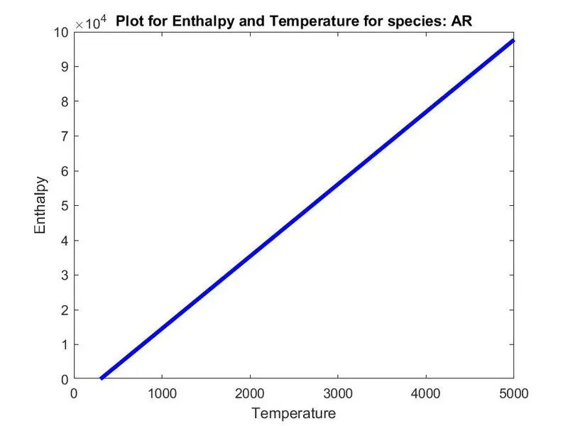
                figure(2)
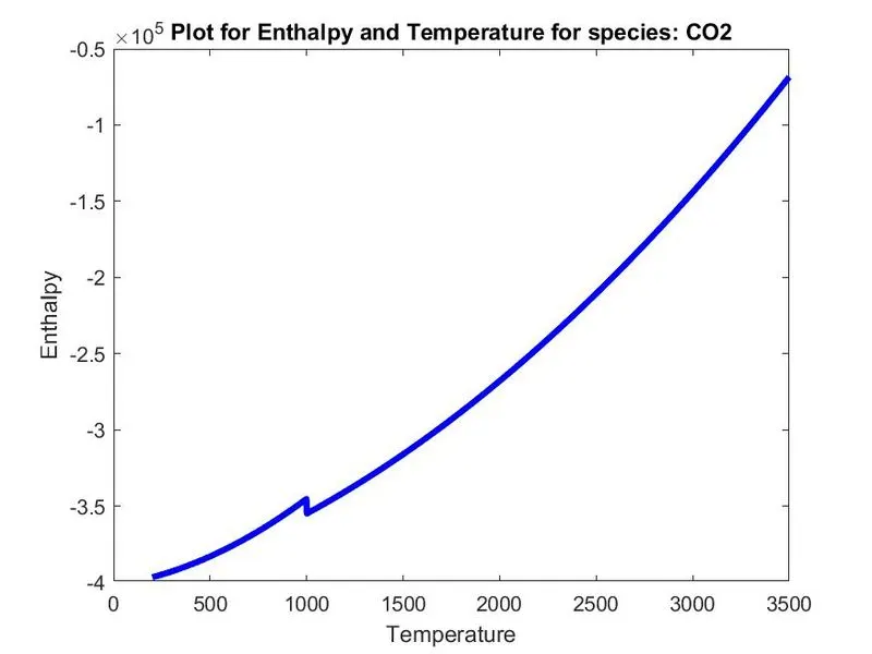
                plot(t_array,h,'linewidth',3,'color','b')
                xlabel('Temperature')
                ylabel('Enthalpy')
                title(sprintf('Plot for Enthalpy and Temperature for species: %s', species_name))
                saveas(figure(2),'Temperature Vs Enthalpy.jpg')

                figure(3)
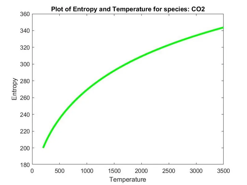
                plot(t_array,s,'linewidth',3,'color','g')
                xlabel('Temperature')
                ylabel('Entropy')
                title(sprintf('Plot of Entropy and Temperature for species: %s', species_name))
                saveas(figure(3),'Temperature Vs Entropy.jpg')

 %   To redirect MATLAB to a directory where the function is saved
 %   Previously the directory of matlab had been changed to a new folder called Plots
 %   In 'Plots' all the plots had been saved with respect to each compound
    cd('D:\krishnaprograms')

    disp(species_name)

 %   Function call
    [total_m_wt]= molecular_weight(species_name)

 %   To remove unwanted trivial warning messages in the console
    warning('off','all')
 end
FUNCTION CODE :
function total_m_wt = molecular_weight(species_name)

   element = {'O','C','H','Ar','N','S'};

   Atomic_mass = [15.99,12.01,1.00,39.94,14.00,32.06];

   total_m_wt = 0;

   for i = 1:length(species_name)
       for j = 1:length(Atomic_mass);
           if strcmpi(species_name(i),element(j));
           total_m_wt = total_m_wt + Atomic_mass(j);
           q=j;
           end
       end
       m = str2double(species_name(i));
       if m>1
            total_m_wt =  total_m_wt+(Atomic_mass(q)*(m-1));

      end
   end
REASULT: The below image shows separate folders for each species with suitable name. which is Generated Automatically
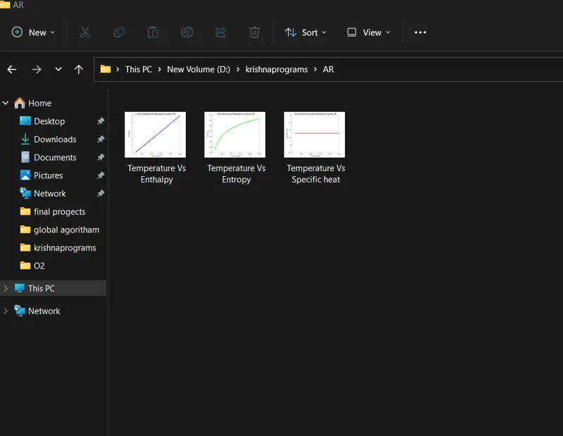
The Below image shows the contents of first species folder (AR) Argon gas
The below image shows the plot of Temp vs Specific Heat of Argon gas
The below image shows the Plot of Temp Vs Enthalpy of Argon gas
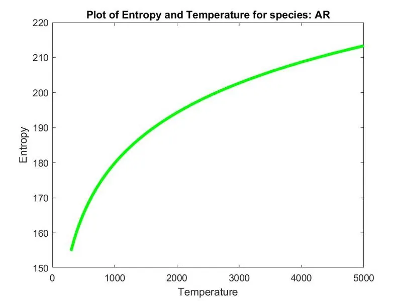
The below image shows the Plot of Temp Vs Entropy of Argon gas
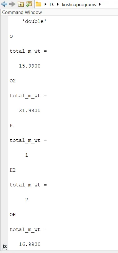
The below image shows the Each Species name and it's Molicular weight.
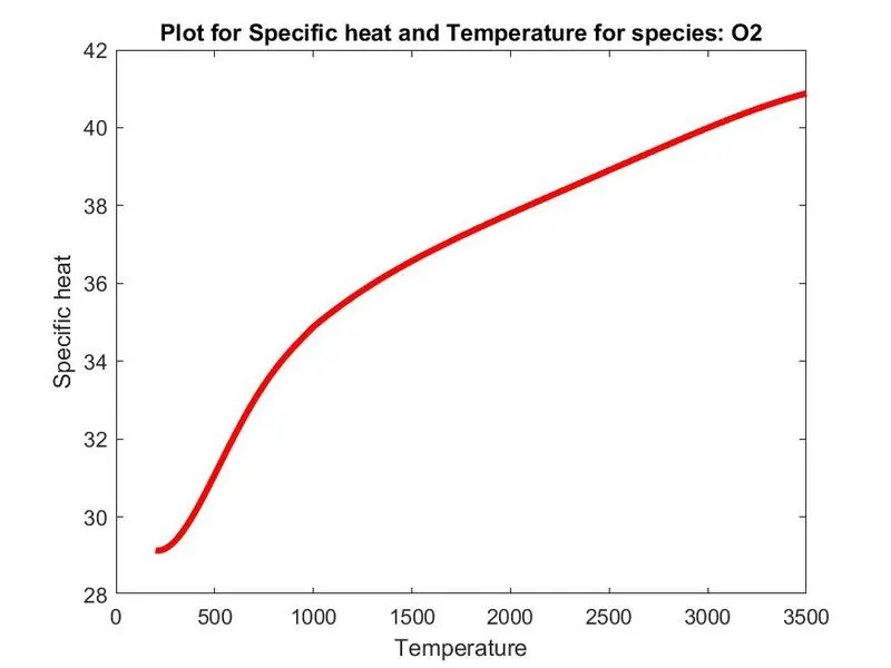
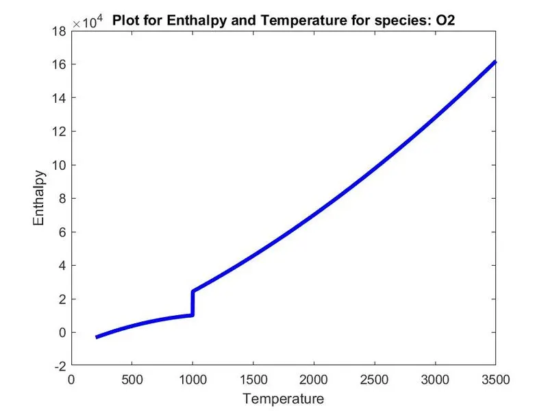
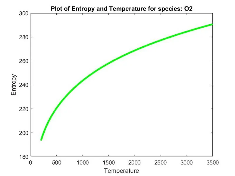
The below 3 figures shows the variation of temp vs CP,H,S in (O2)
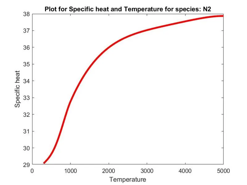
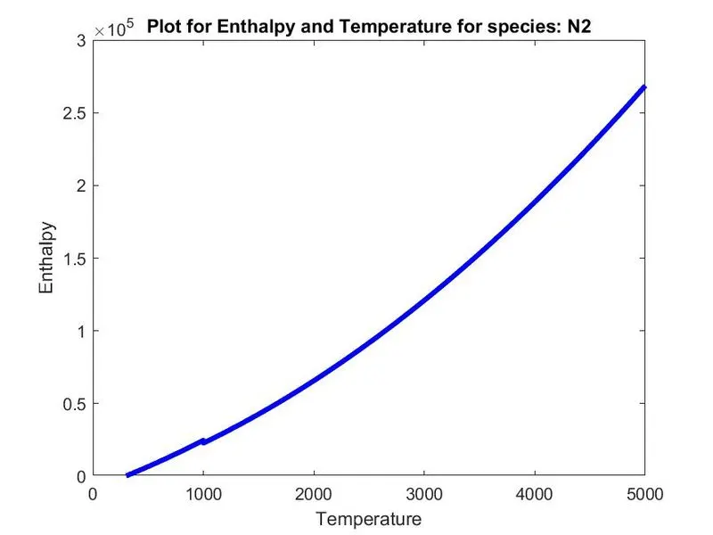
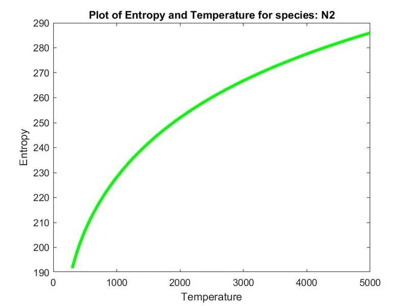
The below 3 figures shows the variation of temp vs CP,H,S in (N2)
The below 3 figures shows the variation of temp vs CP,H,S in (CO2)