Solving second order ODEs

import numpy as np
from scipy.integrate import odeint
import matplotlib.pyplot as plt
import math

#function that return dz/dt
def model(theta,t,b,g,l,m):

theta1=theta[0]
theta2=theta[1]
dtheta1_dt= theta2
dtheta2_dt= -(b/m)*theta2-(g/l)*math.sin(theta1)
dtheta_dt= [dtheta1_dt, dtheta2_dt]
return dtheta_dt

b=0.02
g=9.81
l=1
m=0.1

#initial condition
theta_0 = [0,5]

# time points
t = np.linspace(0,10,150)

# solve ODE
theta = odeint(model,theta_0,t,args = (b,g,l,m))

#plot results

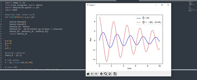
plt.plot(t,theta[:,0], 'b-', label=r'$frac{dtheta_1}{dt}=theta2$')
plt.plot(t,theta[:,1],'r--', label=r'$frac{dtheta2}{dt}=-frac{b}{m}theta_2-frac{g}{L}sintheta_1$')
plt.ylabel('Plot')
plt.xlabel('time')
plt.legend(loc='best')
plt.show()

#animation

THETA3=[]
for theta3 in theta[: , 0]:
THETA3.append(theta3)

ct=1
for THETA4 in THETA3:
x0=0
y0=0

x1=l*math.sin(THETA4)
y1=-l*math.cos(THETA4)
filename='Pendulum%05d.png'%ct
ct=ct+1
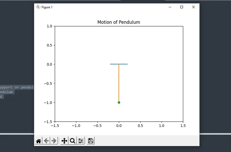
plt.plot([-0.2,0.2],[0,0]) #horizontal support or pendulum
plt.plot([x0,x1],[y0,y1]) #string of pendulum
plt.plot(x1,y1,'-o') #bob tied at the end
plt.xlim([-1.5,1.5])
plt.ylim([-1.5,1])
plt.title('Motion of Pendulum')
plt.savefig(filename)
plt.show()

Explanation:

1) To solve the ode module import odeint module from scipy module

2) Break down the ode into the first two-order ode, the first-order ode will be displacement and the second-order ode will be the value of ode.

3) define the initial conditions to solve the ODE as theta_0 = [0,3]

4) To obtain the smooth motion divide the point from 0 to 20 using linspace command

5) To solve the ode use ODEINT

theta = odeint(model,theta_0,t,args = (b,g,l,m))

6) First column of matrix represents value of displacement hence extracted value of displacement and add it in the null matrix THETA3 using append command

7) To show the motion pendulum for every value THETA3 extract the THETA4 using for loop.