Ahmed Body

Simulating the flow over an Ahmed Body in ANSYS FLUENT

Introduction

Ahmed Body

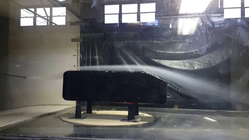
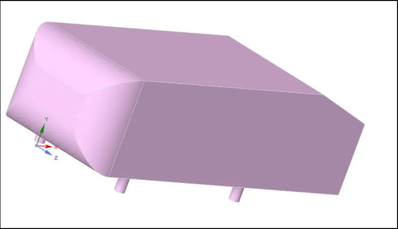
Ahmed's body is a three-dimensional model of an aerodynamic vehicle prototype that has the same shape as a genuine vehicle. R. S. Ahmed initially proposed it in his 1984 paper "Some Salient Features of the Time-Averaged Ground Vehicle Wake." It has since become a standard for aerodynamics simulation software. The length of the simple geometrical shape is 1.04 m, with a height of 0.288 m and a width of 0.389 m. It also includes 0.5 m cylindrical legs attached to the bottom of the body d and a 40-degree slope on the back surface.

The body is in the shape of a highly simplified automobile, with a blunt nose with rounded corners attached to a box-like central part and the ear, as well as a slanted surface (similar to a hatchback car), the angle of which is specified by the engineer in our instance at roughly 40 degrees.

Significance

It's employed in the automotive industry's aerodynamics areas to investigate the impact of the floor pattern on the drive. The external aerodynamics of a car dictate any important characteristics of a vehicle, such as stability, comfort, and fuel efficiency at high speeds. Extreme turbulence and three-dimensional flow separations characterize the flow surrounding the vehicle, as well as growing demand for the most thorough understanding of physical features and dynamical flow. It is used to investigate flow analysis and determine how much weight moves around the body.

The primary goal of studying such a basic automobile body is to investigate the flow dynamics involved in drag creation. By anticipating the mechanisms that cause drag, an automobile can be designed to reduce drag and hence reduce fuel consumption while maximizing vehicle performance.

It is also used to determine track force, left force analysis, rolling pitching, yawing, and during moments, in addition to the velocity field.

Negative Pressure in Wake Region

When the air flowing over a vehicle is separated at the back end, a big low-pressure turbulent zone known as ‘wake’ is left behind the vehicle. The vehicle's performance compensates for the pressure drag caused by this wake.

This region of recirculating flow straightaway behind a moving or a stationary blunt-body is caused by viscosity, which can be amid flow separation and turbulent flow, or the wave pattern on the water surface downstream of an object during a flow, or created by a moving object, caused by density distinction in a fluid higher than and below the free surface and gravity.

When the car is moving at a velocity, the vicious impact withinside the fluid is constrained to a skinny layer known as the boundary layer. Outside the boundary layer is the inviscid float. This fluid float imposes strain pressure at the boundary layer. When the air reaches the rear part of the car, the fluid becomes detached. Within the boundary layers, the motion of the fluid is ruled with the aid of using the vicious impact of the fluid.

The Reynolds number depends on the characteristic length of the vehicle, the kinematic viscosity of the air and therefore the speed of the vehicle. The fluid travelling the vehicle depends on the form of the vehicle and therefore the Reynolds number. There's another important phenomenon, which affects the ground of the air around the car and therefore the performance of the vehicle. This phenomenon is usually referred to as the 'Wake' of the vehicle. When the air moving over the vehicle is separated at the buttocks, it leaves an outsized low-pressure turbulent region behind the vehicle referred to as wake. This wake contributes to the formation of pressure drag, which is eventually reducing the vehicle performance.

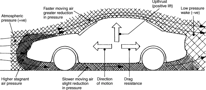
As shown above,

Significance of the Point of Separation

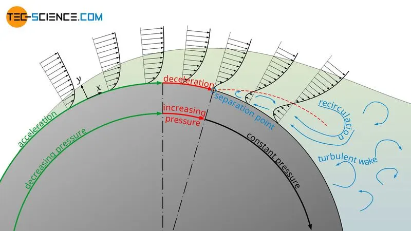
Separation of flow is said to occur when the direction of flow velocity near the surface is opposite to the direction of free stream velocity. Which means (du/dy) ≤ 0. Such a situation arises when there is a negative pressure gradient near the wall.

In the direction of the flow the pressure increases which causes a decrease in velocity and creates conditions for separation to occur. It is important to know that the skin friction condition reaches zero. This point where the wall shear stress vanishes is called the separation point. Reverse flow takes place beyond the point of separation. Due to reverse flow, irregular eddies are formed and a lot of energy is dissipated. This region is called 'Wake'. The pressure distribution in the wake is quite different from that on the remaining boundary and this gives rise to additional drag force on the body. Wake also leads to lateral vibration to the object which may be harmful. Also, a large amount of kinetic energy is lost.

Problem

As the body is perfectly symmetric, we can simulate by considering the only half body. This is the best practice where you can save on the number of cells and get the results faster as well.

Simulate the velocity of 25 m/sec with the default air properties in fluent.

For this challenge, you will have to provide answers to the following questions:

Q1. Describe Ahmed's body and its importance.

Q2. Explain the reason for the negative pressure in the wake region.

Q3. Explain the significance of the point of separation.

Expected Results:

1. Velocity and pressure contours.

2. The drag coefficient plot for a refined case. ( For a velocity of 25m/sec, the drag coefficient should be around 0.33).

3. The vector plot clearly shows the wake region.

4. Perform the grid independence test and provide the values of drag and lift with each case.

Solution

Geometry

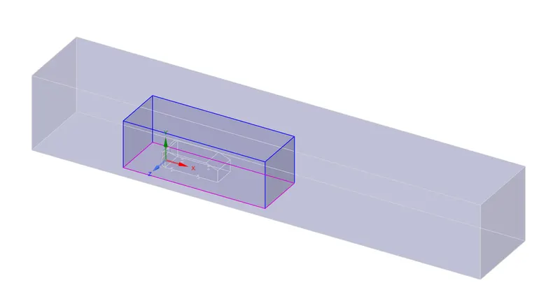
The geometry of the Ahmed body is loaded into SpaceClaim. The Ahmed body is enclosed in a controlled space that acts as a wind tunnel. Around the body a second control space is generated is called Local Refinement volume where the mesh is a lot final then the rest of the volume this region of refinement is determined iteratively.

Mesh

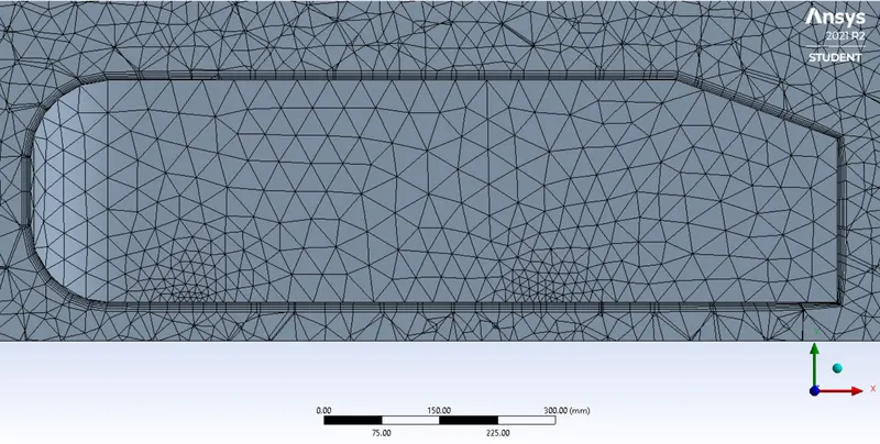
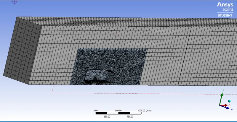
under these circumstances, we use multiZone mesh on the outer control volume and a super fine prismatic mash on the inner Local Refinement volume. The MultiZone mesh has a high quality all match types and divides the control volume into small cubes.

Around Ahmed body cavity we build an inflation layer to increase the quality of output and all the boundary conditions are mentioned

The meshing will be divided into 3 cases;

Setup

Case 1.1:

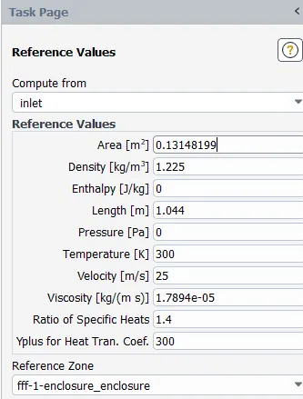
We first perform a quality check on the Mesh and then set up the physics for the solution. The solver chosen is the pressure-based solver. And the viscosity model is the K-ε model.

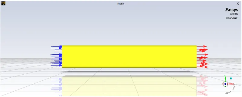
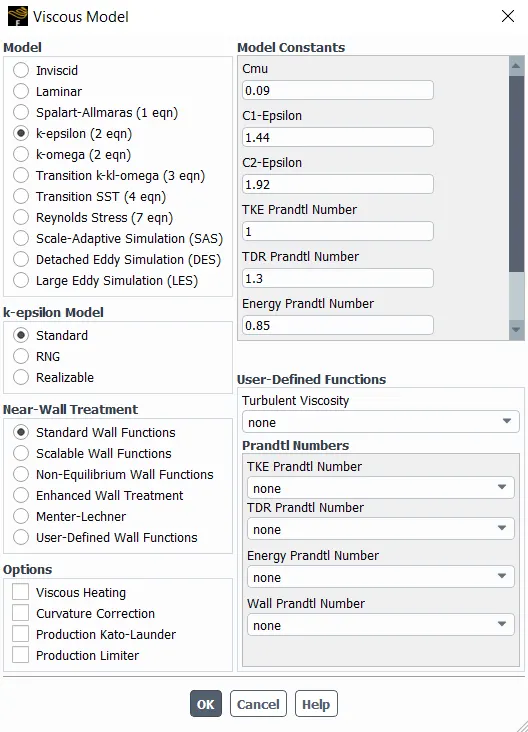
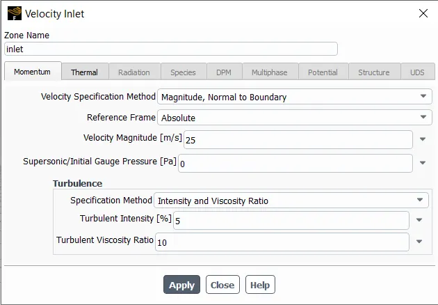
With these inputs, we will ‘Initialise’ the solver and simulate 500 iterations.

The first plot is the scaled residuals,

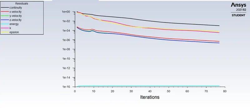
Scaled Residuals

This is followed by the drag coefficient plot,

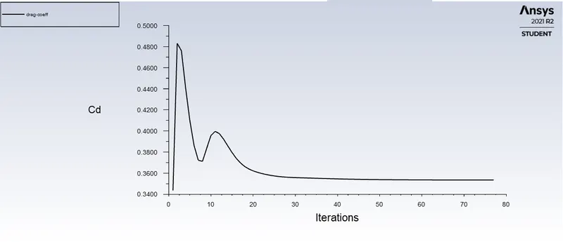
Drag Coefficient

Followed by Lift coefficient plot,

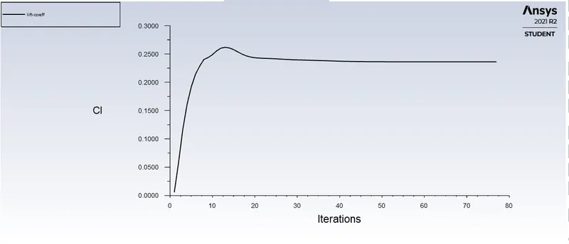
Lift Coefficient

And we will generate the contour diagrams of the model and study the velocity and pressure profiles and observe the velocity with the help of vectors.

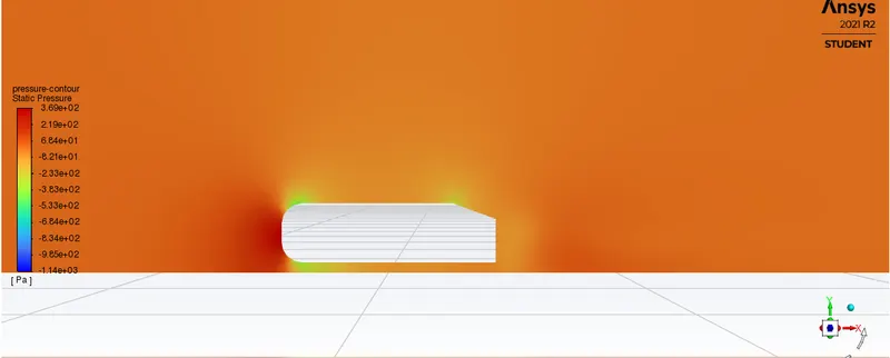
Pressure contour,

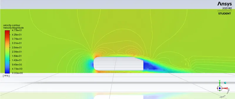
Velocity Contour, velocity vector plot.

Case 1.2:

We first perform a quality check on the Mesh and then set up the physics for the solution. The solver chosen is the pressure-based solver. And the viscosity model is the K-Ω model.

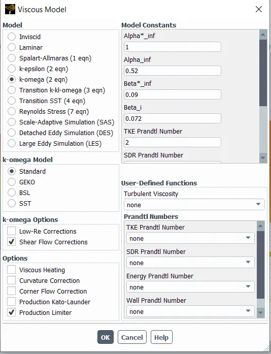
With these inputs, we will ‘Initialise’ the solver and simulate 500 iterations.

The first plot is the scaled residuals,

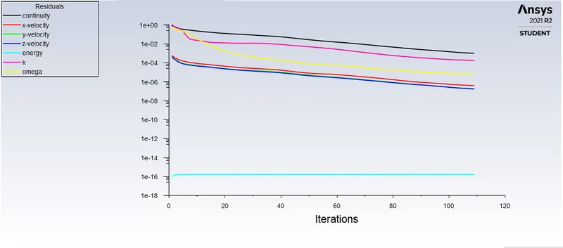
Scaled Residuals

This is followed by the drag coefficient plot,

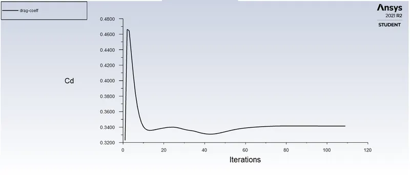
Drag Coefficient

Followed by Lift coefficient plot,

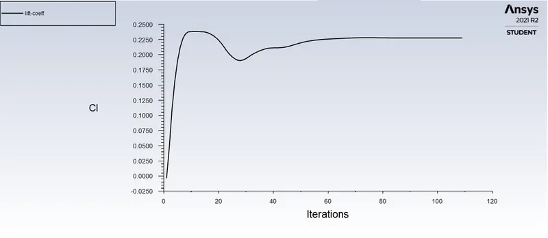
Lift Coefficient

And we will generate the contour diagrams of the model and study the velocity and pressure profiles and observe the velocity with the help of vectors.

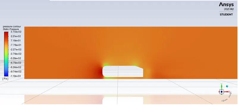
Pressure Contour,

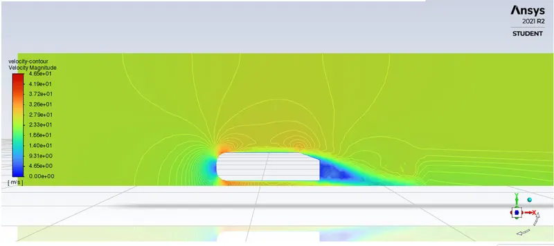
Velocity Contour and Velocity vector plot,

Case 2.1:

We first perform a quality check on the Mesh and then set up the physics for the solution. The solver chosen is the pressure-based solver. And the viscosity model is the K-ε model.

With these inputs, we will ‘Initialise’ the solver and simulate 500 iterations.

The first plot is the scaled residuals,

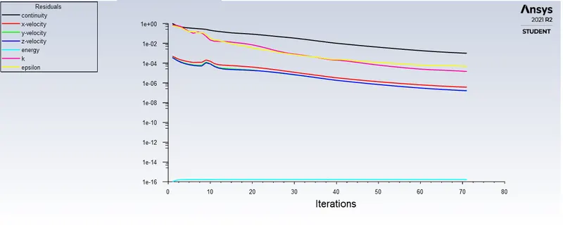
Scaled Residuals

This is followed by the drag coefficient plot,

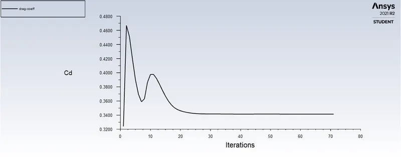
Drag Coefficient

Followed by Lift coefficient plot,

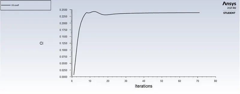
Lift Coefficient

And we will generate the contour diagrams of the model and study the velocity and pressure profiles and observe the velocity with the help of vectors.

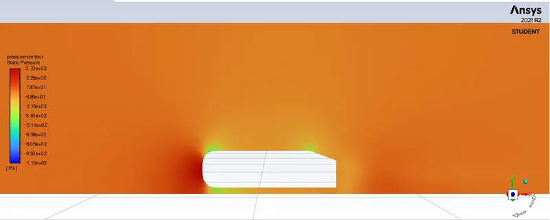
Pressure Contour,

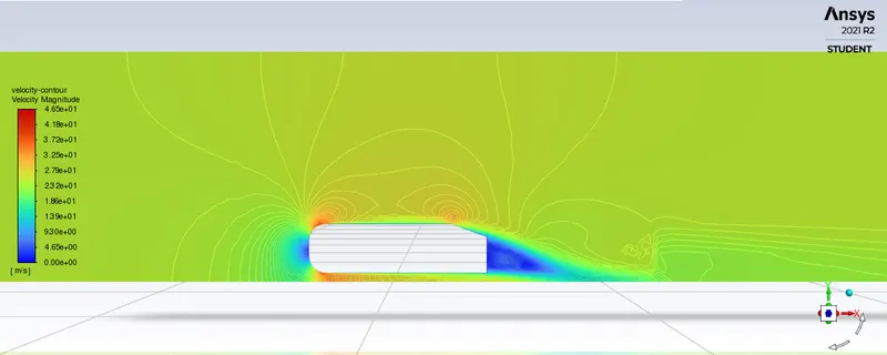
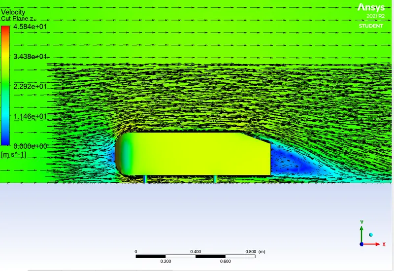
Velocity Contour, velocity vector plot.

Case 2.2:

We first perform a quality check on the Mesh and then set up the physics for the solution. The solver chosen is the pressure-based solver. And the viscosity model is the K-Ω model.

With these inputs, we will ‘Initialise’ the solver and simulate 500 iterations.

The first plot is the scaled residuals,

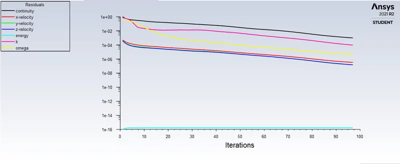
Scaled Residuals

This is followed by the drag coefficient plot,

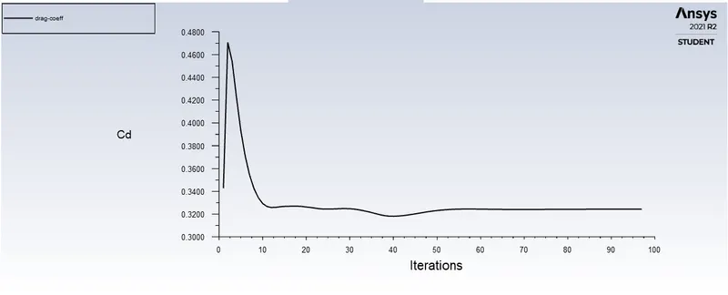
Drag Coefficient

Followed by Lift coefficient plot,

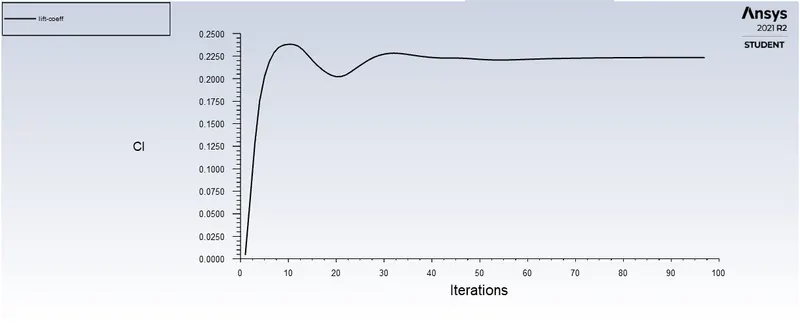
Lift Coefficient

And we will generate the contour diagrams of the model and study the velocity and pressure profiles and observe the velocity with the help of vectors.

Pressure Contour,

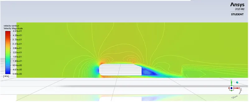
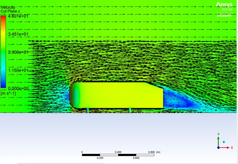
Velocity Contour, velocity vector plot.

Case 3.1:

We first perform a quality check on the Mesh and then set up the physics for the solution. The solver chosen is the pressure-based solver. And the viscosity model is the K-ε model.

With these inputs, we will ‘Initialise’ the solver and simulate 500 iterations.

The first plot is the scaled residuals,

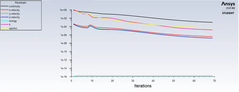
Scaled Residuals

This is followed by the drag coefficient plot,

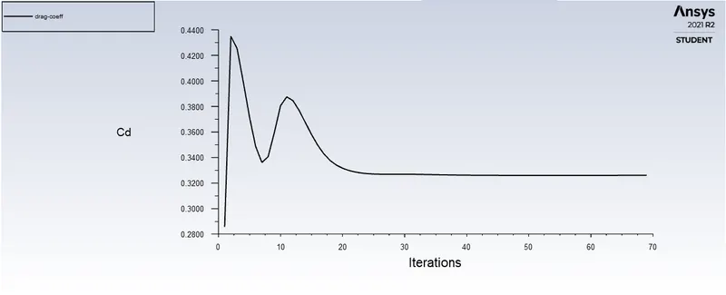
Drag Coefficient

Followed by Lift coefficient plot,

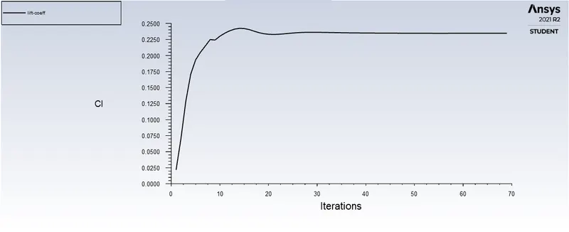
Lift Coefficient

And we will generate the contour diagrams of the model and study the velocity and pressure profiles and observe the velocity with the help of vectors.

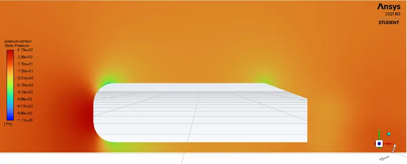
Pressure Contour,

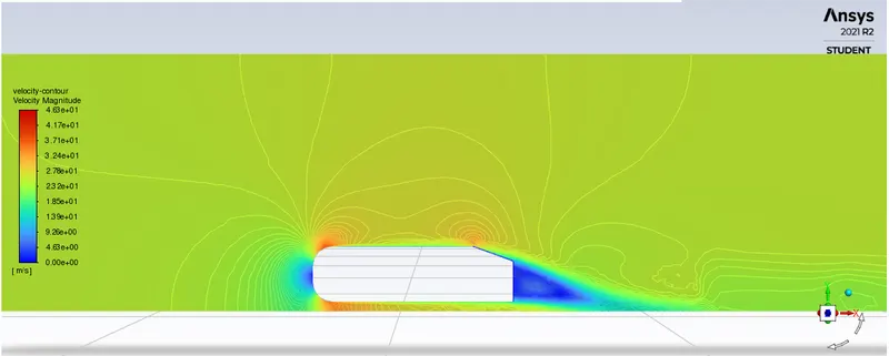
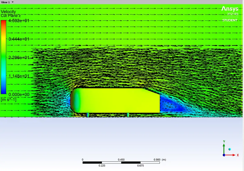
Velocity Contour, velocity vector plot.

Case 3.2:

We first perform a quality check on the Mesh and then set up the physics for the solution. The solver chosen is the pressure-based solver. And the viscosity model is the K-Ω model.

With these inputs, we will ‘Initialise’ the solver and simulate 500 iterations.

The first plot is the scaled residuals,

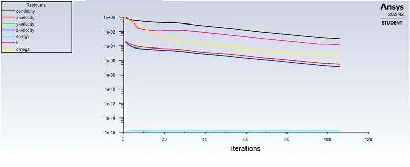
Scaled Residuals

This is followed by the drag coefficient plot,

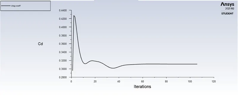
Drag Coefficient

Followed by Lift coefficient plot,

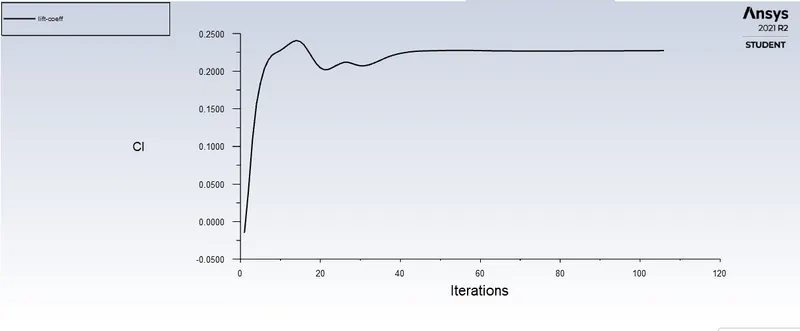
Lift Coefficient

And we will generate the contour diagrams of the model and study the velocity and pressure profiles and observe the velocity with the help of vectors.

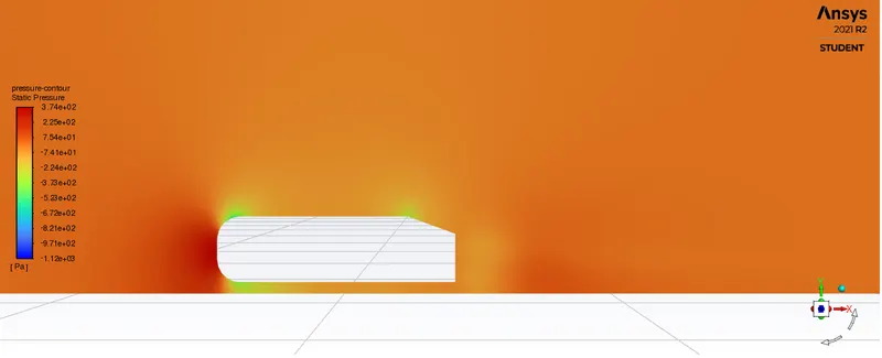
Pressure Contour,

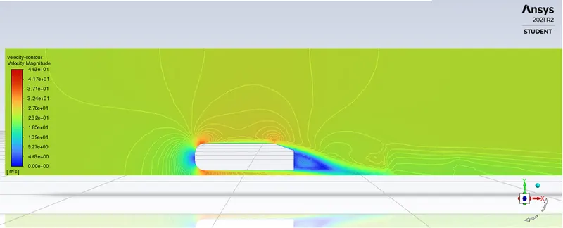
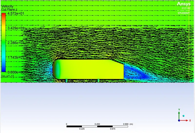
Velocity Contour, velocity vector plot.

Conclusion

• By iterating several steady-state simulations, performing a mesh dependency test with three cases on Ahmed body, obtaining significant convergence according to velocity, drag and lift coefficients, for each case, to a quasi-steady result.
• The great dependency test proves that finer mesh gives more accurate results.
• Another important result that was concluded was that the K-Ω model gives better results than the K-ε model, also it was found that K-Ω takes more iterations to solve the convergence but it gives good results.
• With the increased refinement the reduction in drag coefficient and increment in lift coefficient is observed.
• When the CFD results are compared to the experimental result, all the cases are close to the experimental results.

Report Link: https://docs.google.com/document/d/1cKHCGAHQhegmimziLp1lXLq-gtbsvVPYKezeTqeSd_o/edit?usp=sharing