Flow Over a Cylinder

Using ANSYS FLUENT to Simulate Flow Over a Cylinder

Introduction

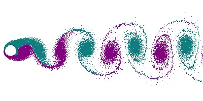
When fluid flows around a cylindrical object, there is a range of flow velocities for which a Von Karman Vortex street is formed. For the velocities exceeding the laminar flow, the inertia of the fluid becomes significant and, as the fluid stream passes the front most of the cylinder, it is unable to negotiate the rear half of the cylinder, Hence the fluid tends to separate from the front surface and peels off as it approaches the rear end of the cylinder, ending up shedding the vortex

Karman Vortex Street is a repeating pattern of swirling vortices, caused by a process known as shedding. Which is responsible for the unsteady separation of most of the flow around blunt bodies.

Vertex shading is an oscillating flow that takes place when a fluid such as air or water flows past a certain body at a certain velocity, depending on the size and shape of the body.

During this flow, vortices are created at the back end of the body forming a von Karman vortex Street which is responsible for the unsteady separation of flow of the fluid around the blunt-body.

The fluid flow past the object creates alternating low-pressure vortices on the downstream side of the object. The object will tend to move towards the low-pressure zone hence creating a whirling-type motion.

Reynolds number, A dimensionless number that plays an important role in problems concerning flow, is the ratio of internal forces to the viscous forces,

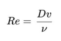
• Used in forced convection, all types of heat transfer in which the fluid is forced to move to increase heat transfer.
• The Reynolds number predicts the flow pattern.
• The laminar flow is achieved due to low Reynolds number and the turbulent flow is achieved due to high Reynolds number.

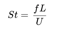
Strouhal number, A dimensionless number/ parameter which is used to describe the oscillating flow mechanism.

With the parameter, we can determine which model of flow will be dominant. The ratio of internal forces due to the unsteadiness of the flow or local acceleration to the inertial forces due to changes and velocity from one point to another in the flow field.

Problem

1. Simulate the steady and unsteady flow and calculate the Strouhal number for Re = 100;
2. Calculate the coefficient of drag and the lift coefficient, over a cylinder by setting up the Reynolds number to be 10, 100, 1000, 10000, and 100000 (Run with the steady solver),
3. Study the effect of Reynolds number on the drag coefficient,

Solution

Geometry

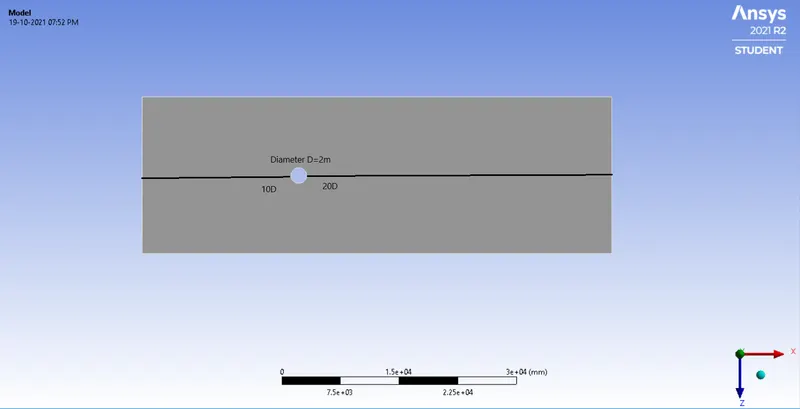
With the CAD Cleanup and SpaceClean, we define the geometry of the computational domain.

Mesh

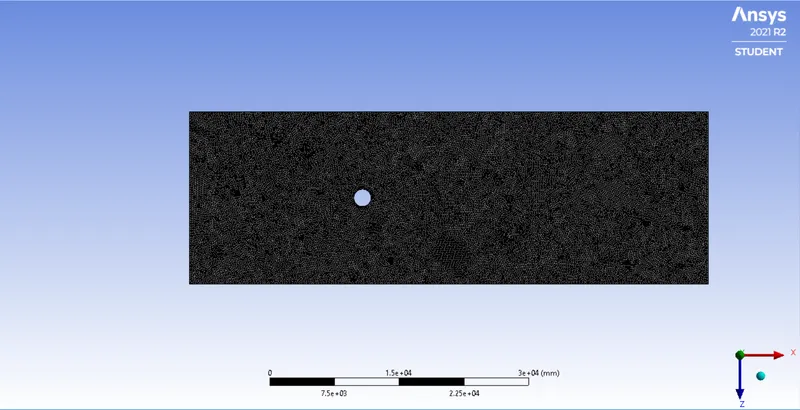
Once the geometry is set up we will generate the mesh for the geometry, the mesh we will use is a triangular mesh and the mesh around the body of concern is highly detailed as the region is the one that will generate the vortices which are to be observed.

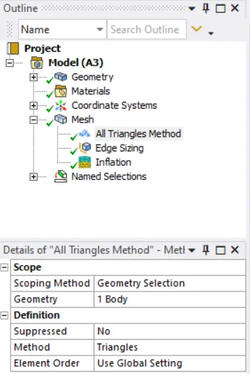
The mesh used is ‘All Triangular Mesh’.

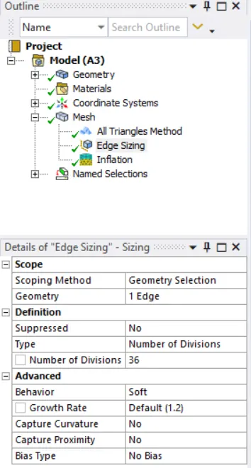
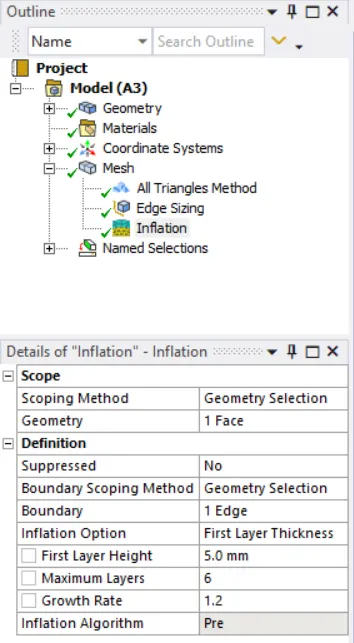
The mesh around the edge is made more detailed by adding edge details, the edge is divided into 36 divisions, and followed by setting up an inflation layer with 6 total layers.

The resulting mesh will be generated as,

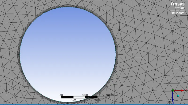
Element size = 200 mm or 0.20 m, 62714 total elements.

Setup

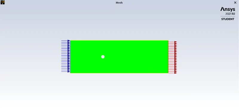
The boundary conditions assigned in the mashing are assigned values and solvers.

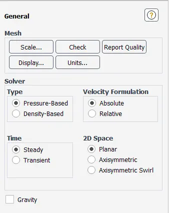
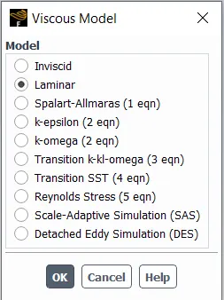
We determine the viscosity model for the system,

The material is edited to be used and the viscosity is changed to 0.02 Kg/m-s and density is 1 Kg/m^3.

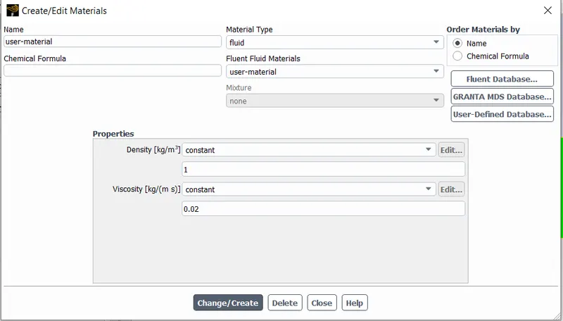
These values and the geometry will remain constant for all the varying values of the Reynolds number.

Setup Re10

Solver- Steady,

Boundary condition-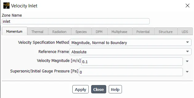

Monitor point is created at the coordinate (x,y)- (8,0)

Reports Generated are Vortex average surface report at the monitor point, Lift coefficient, drag coefficient, Scaler residuals.

Contour Plots for velocity and pressure are generated.

Solution animation is also extracted at every 10 iterations.

Solution Method- SIMPLE

Initialization- Hybrid

No. of iterations- 1000

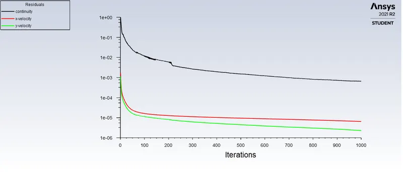
Scaler Residuals

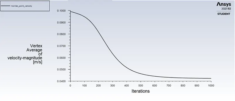
Monitor point velocity,

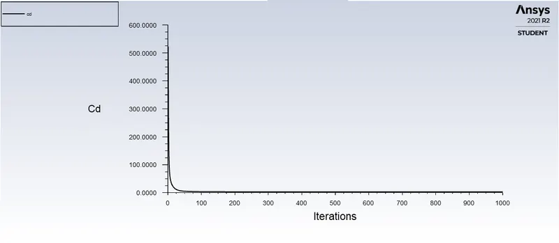
Drag Coefficient, Computed as 3.3291058

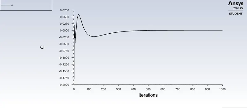
Lift coefficient, Computed as 0.00068707797

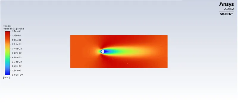
Velocity Contour,

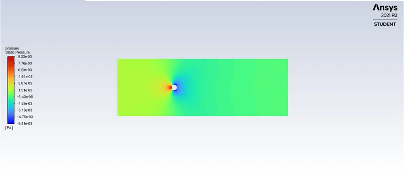
Pressure Contour,

Setup Re 100 Stable

Solver- Steady,

Boundary condition-

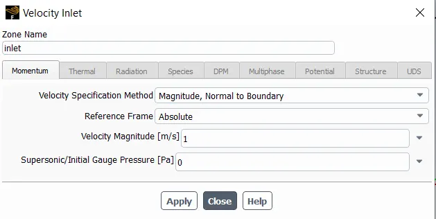
Monitor point is created at the coordinate (x,y)- (8,0)

Reports Generated are Vortex average surface report at the monitor point, Lift coefficient, drag coefficient, Scaler residuals.

Contour Plots for velocity and pressure are generated.

Solution animation is also extracted at every 10 iterations.

Solution Method- SIMPLE

Initialization- Hybrid

No. of iterations- 1000

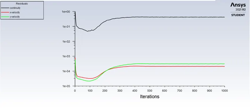
Scaler Residuals,

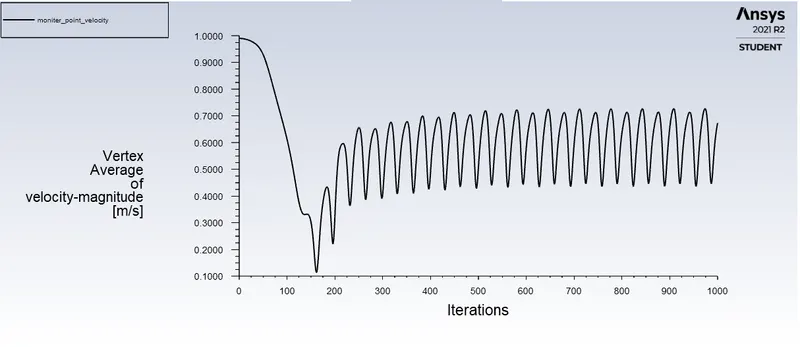
Monitor point velocity,

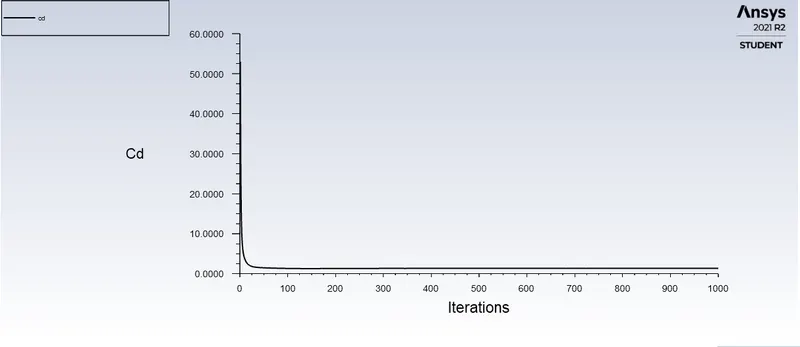
Drag Coefficient, Computed as 1.3546824

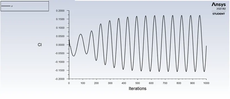
Lift coefficient, Computed as -0.0059364408

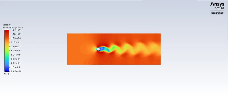
Velocity Contour,

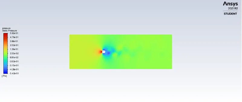
Pressure Contour.

Setup Re 100 Unstable

Solver- Transient,

Boundary condition-

Monitor point is created at the coordinate (x,y)- (8,0)

Reports Generated are Vortex average surface report at the monitor point, Lift coefficient, drag coefficient, Scaler residuals.

Contour Plots for velocity and pressure are generated.

Solution animation is also extracted at every 10 iterations.

Solution Method- SIMPLE

Initialization- Hybrid

No. of iterations- 900

Time step size -0.25 s

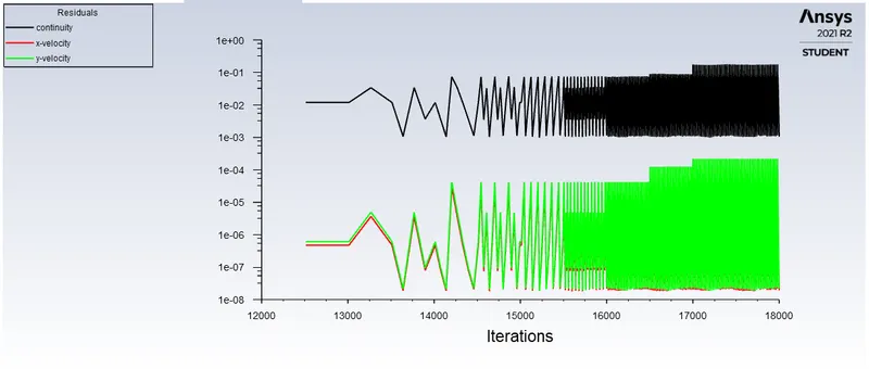
Scaler Residuals,

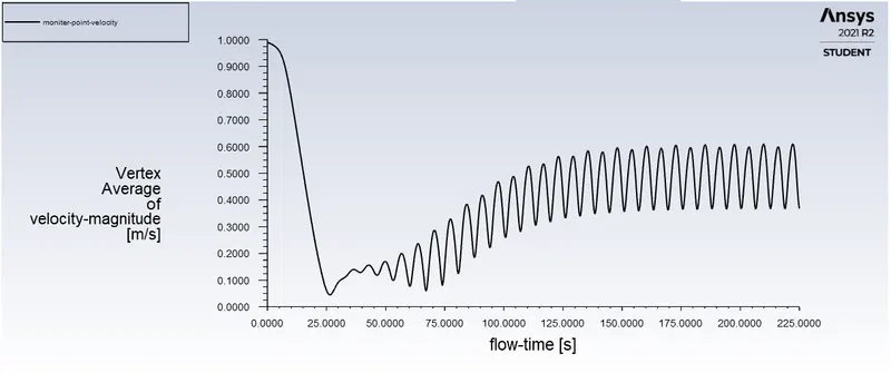
Monitor point velocity,

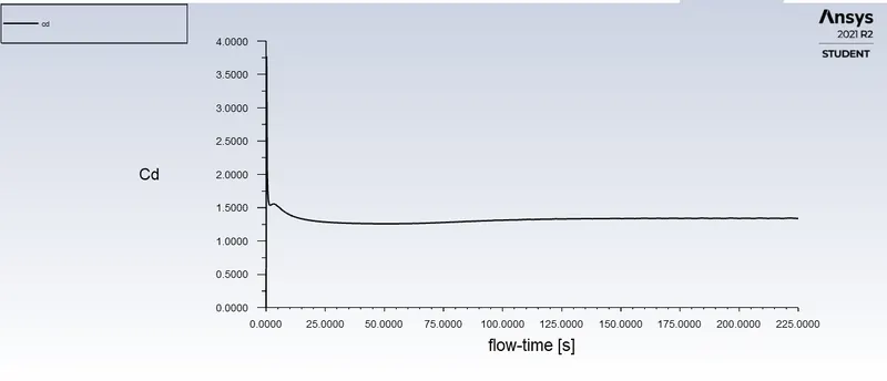
Drag Coefficient, Computed as 1.3400198

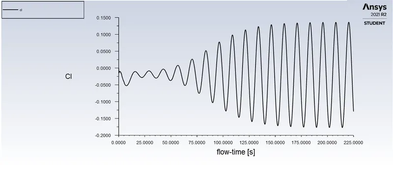
Lift coefficient, Computed as -0.12918268

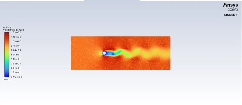
Velocity Contour,

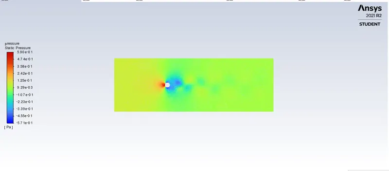
Pressure Contour.

St = f*L/U, Strouhal number for this condition is calculated as shown, f is the frequency of the shedding which is (4/50) = 0.08, L is characteristic length 20m, and U is the flow velocity 1m/s.

St = 0.08*2/1 = 0.16 which is compliant with the theoretical result of 0.15669

Setup Re 1000

Solver- Steady,

Boundary condition-

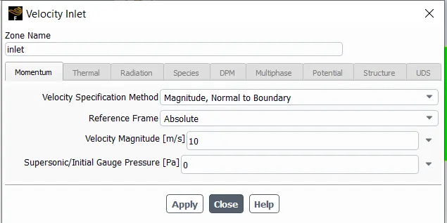
Monitor point is created at the coordinate (x,y)- (8,0)

Reports Generated are Vortex average surface report at the monitor point, Lift coefficient, drag coefficient, Scaler residuals.

Contour Plots for velocity and pressure are generated.

Solution animation is also extracted at every 10 iterations.

Solution Method- SIMPLE

Initialization- Hybrid

No. of iterations- 1000

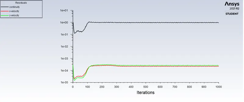
Scaler Residuals,

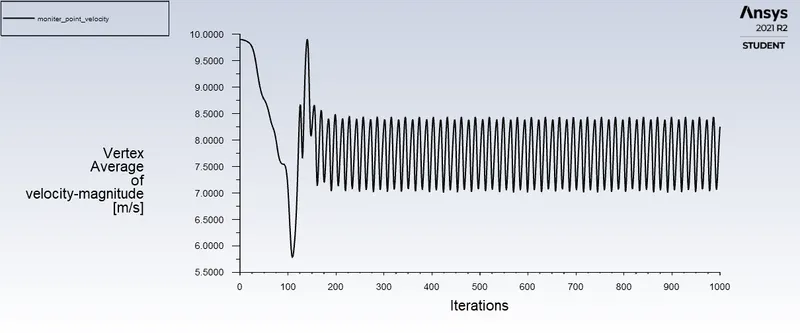
Monitor point velocity,

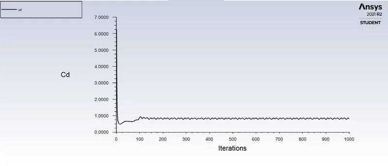
Drag Coefficient, Computed as 0.80881566

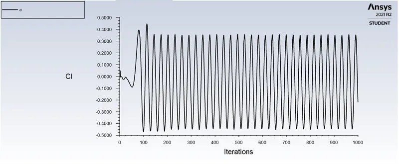
Lift coefficient, Computed as -0.22118129

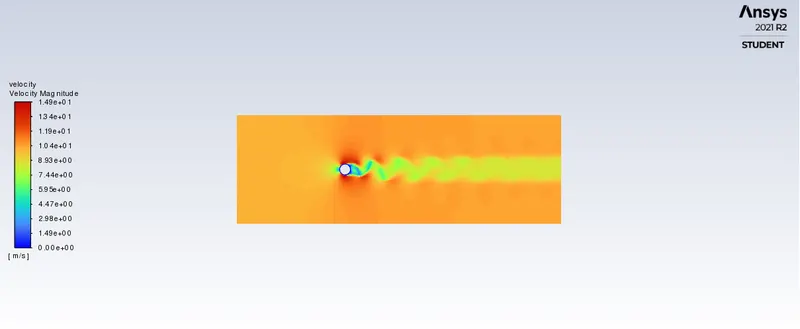
Velocity contour,

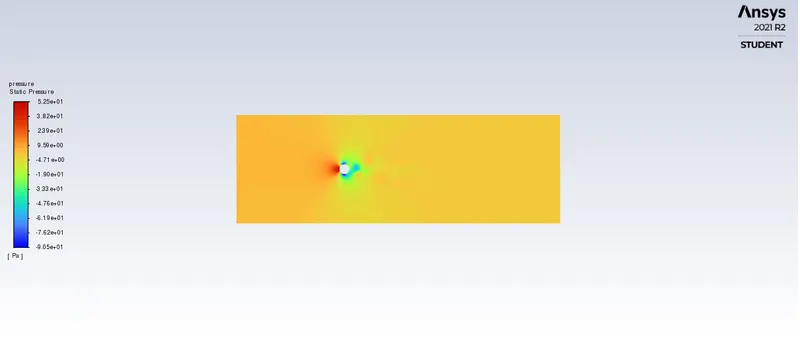
Pressure Contour.

Setup Re 10000

Solver- Steady,

Boundary condition-

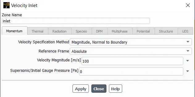
Monitor point is created at the coordinate (x,y)- (8,0)

Reports Generated are Vortex average surface report at the monitor point, Lift coefficient, drag coefficient, Scaler residuals.

Contour Plots for velocity and pressure are generated.

Solution animation is also extracted at every 10 iterations.

Solution Method- SIMPLE

Initialization- Hybrid

No. of iterations- 1000

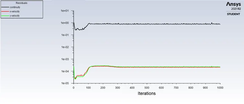
Scaler Residuals,

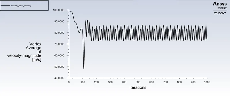
Monitor point velocity,

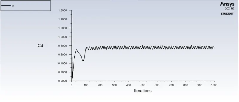
Drag Coefficient, Computed as 0.73705202,

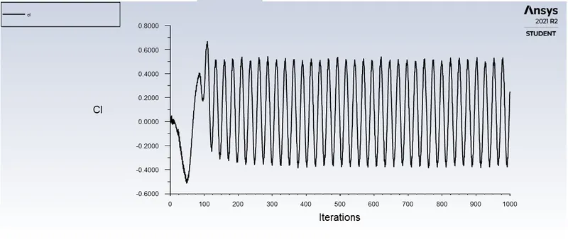
Lift coefficient, Computed as 0.25006069,

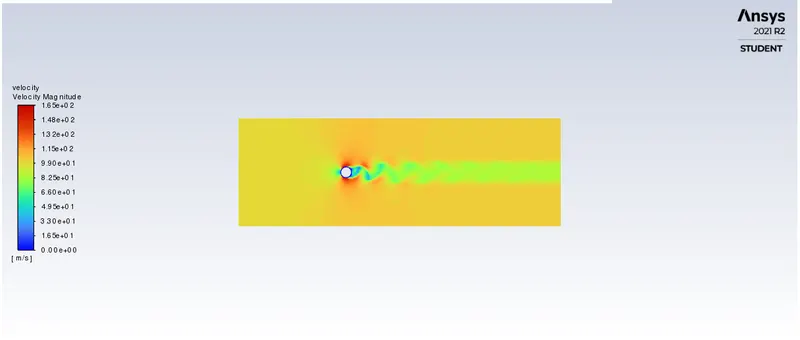
Velocity contour,

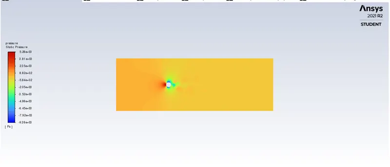
Pressure Contour.

Setup Re 100000

Solver- Steady,

Boundary condition-

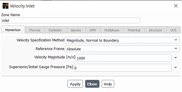
Monitor point is created at the coordinate (x,y)- (8,0)

Reports Generated are Vortex average surface report at the monitor point, Lift coefficient, drag coefficient, Scaler residuals.

Contour Plots for velocity and pressure are generated.

Solution animation is also extracted at every 10 iterations.

Solution Method- SIMPLE

Initialization- Hybrid

No. of iterations- 1000

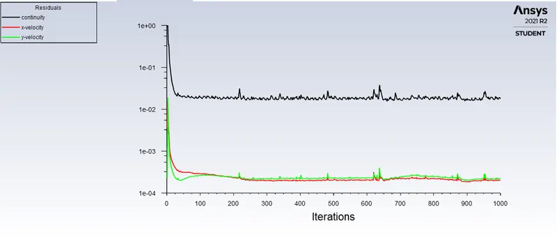
Scaler Residuals,

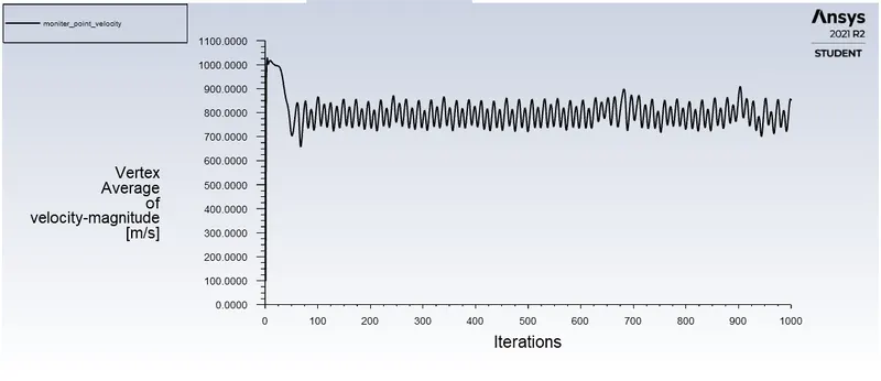
Monitor point velocity,

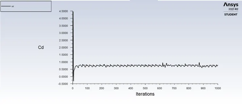
Drag Coefficient,

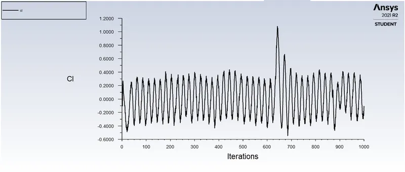
Lift coefficient,

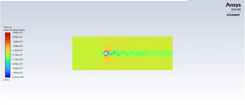
Velocity contour,

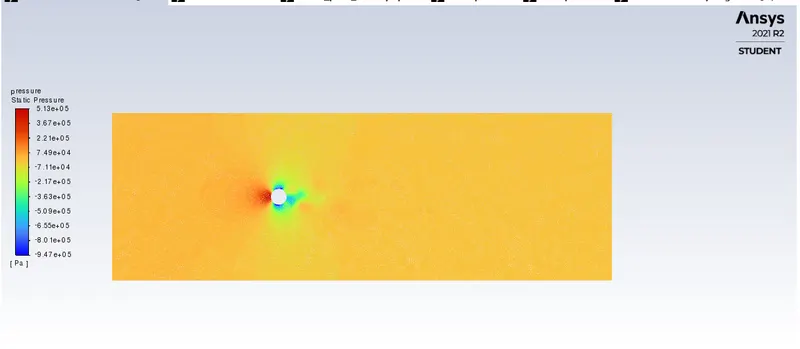
Pressure Contour.

Results and Conclusion

• During the transient state simulation, we are not able to observe any vortex shedding phenomenon at higher time steps, so we lower the time step, increasing the total number of iterations to compute the solution.
• Increasing Reynolds number causes the upper and lower surfaces of the cylinder to shed vortices at particular frequencies.
• At Reynolds numbers below 10, there are no vortices. At Reynolds numbers above 100, vortices begin to shed.
• In comparison to transient state solvers, the steady-state solver has a much higher computation speed.
• The Renault number plays an important role. It depends on geometry, speed, and viscosity, and governs how frequently the vortex sheds.
• Under certain conditions, both transient and steady-state solvers can simulate the expected physics of the flow.

Report Link: https://docs.google.com/document/d/1lORjA9qvdSSfa6LppKijI6KXuDq6HFnSN3YeSUIfnUU/edit?usp=sharing

Video Link: https://youtu.be/HfGSIz2FYPM