1 D Super-Sonic Nozzle Flow

Simulation of 1D Supersonic Nozzle Flow using Maccormack Method

Introduction

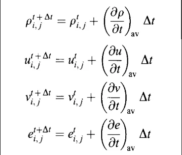
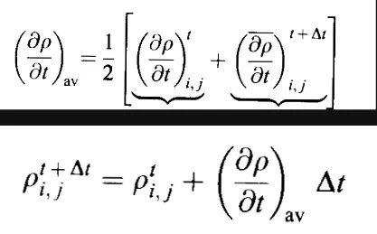
The Maccormack method is a variant of the Lax-Wendroff method. We use this method so that we can avoid the use of second-order derivatives. Instead, an average of the first derivative is used (calculated by forwarding difference scheme and backward scheme).

(∂ ρ / ∂ t )av derived by predictor and corrector philosophy.

Predictor Step

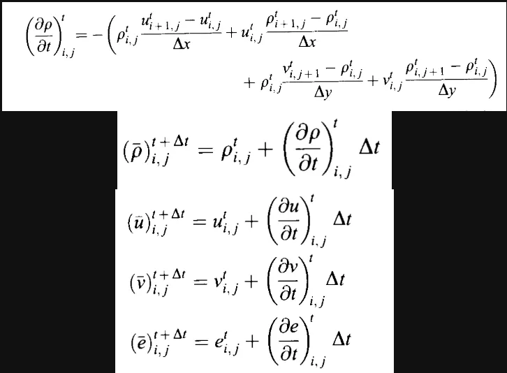
The governing equation is discretized in a forward skewed scheme and marched in time.

Corrector step

In this step, the ideology mostly remains the same as the governing equation march in time but the backward difference is used in the spatial derivative.

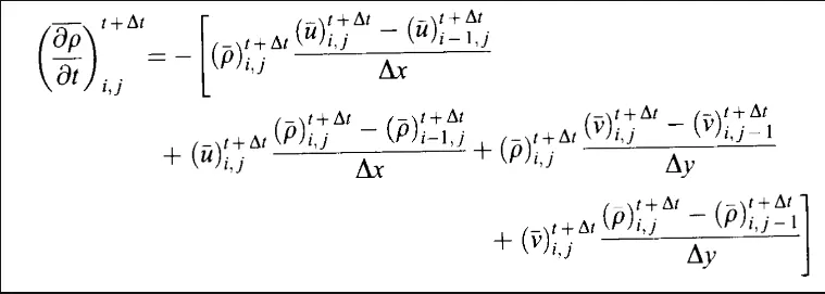
We take an average of both the time derivatives calculated from the above-mentioned methods, and the average is used in the calculator of the results for every grid point while marching forward in time.

One Dimensional Nozzle Flow

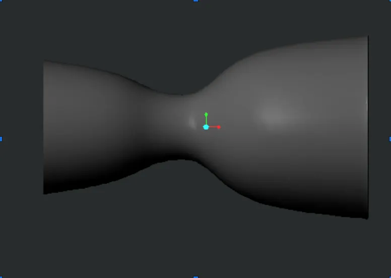
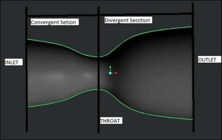
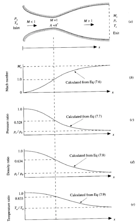
The flow expands isentropically to supersonic speeds at the nozzle exit. The flow is locally subsonic in the convergent sections of the nozzle, sonic at the throat, and supersonic at the divergent section.

The flow properties mostly remain uniform across the section, despite the change in the area concerning the distance along ‘x’. Therefore we assume that the flow properties vary only in the x-direction

When we consider the geometrical aspects and the flow properties along with the geometry we see that the flow at the inlet of the nozzle comes from the reservoir where the pressure and temperature are denoted by Po and T o respectively. At the same time, the inlet velocity is very small making Po and T o stagnant values.

Three important regions of focus are;

1. Convergent section of the nozzle where the Mach number is less than 1 and the flow is Subsonic.
2. The throat of the nozzle where the local velocity is equal to the local speed of sound and the flow is Sonic.
3. The divergent section where the Mach number is greater than one and the flow is Supersonic.

Problem Question

Simulate isentropic quasi 1 D subsonic-supersonic nozzle flow. Using the Maccormack method derivation the conservative and non-conservative form of governing equation. Determination of steady-state temperature distribution for the flow field variables and investigate the difference between the 2 forms of governing equation by comparing the results.

Solution

Physical Appearance and the Assumption of the Flow

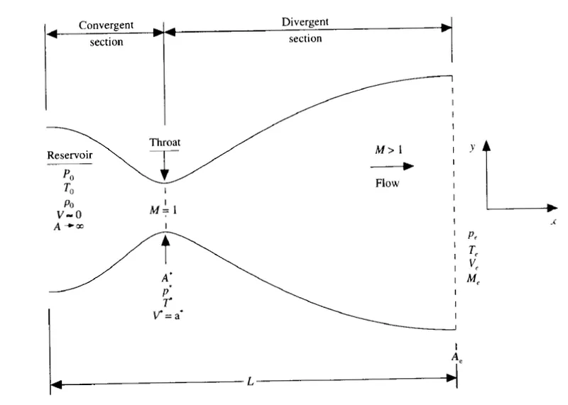
We consider the steady isentropic flow through a convergent-divergent nozzle as represented, Source at the nozzle inlet is considered from a reservoir, where the pressure and temperature are denoted by Po and T o respectively. The area of the reservoir is considered to be a very large limit of A-> infinity, which leads the velocity at the inlet to be very small, almost 0. Making Po and T o stagnant values. The sections can be assumed to be separated into 3 zones of concern.

Three important regions of focus are;

1. Convergent section of the nozzle where the Mach number is less than 1 and the flow is Subsonic.
2. The throat of the nozzle where the local velocity is equal to the local speed of sound and the flow is Sonic.
3. The divergent section where the Mach number is greater than one and the flow is Supersonic.

Assumptions

A cross-section area A, where the flow properties are uniform across the section. The area of the nozzle changes as a function of distance along with the nozzle, x, which logically makes the problem a 2D flow field problem, but we assume the flow properties are only dependent on ‘x’. Which makes the problem by definition a quasi-one-D flow problem.

Governing Equation (Analytical solution)

The governing continuity, momentum, and energy equations for this quasi-one-dimensional, steady, isentropic flow can be expressed, respectively, as

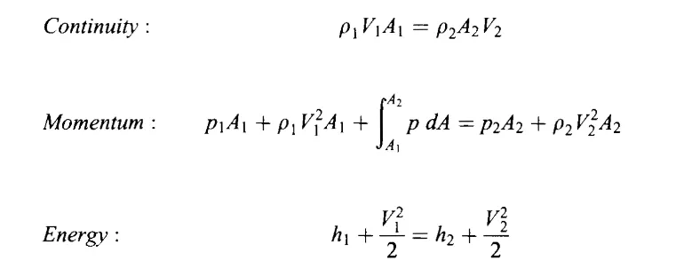
where subscripts I and 2 denote different locations along with the nozzle. In addition, we

have the perfect gas equation of state,

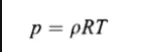
as well as the relation for a calorically perfect gas,

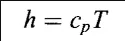
Since we already have results for the given problem then we can use this to test the application of the CFD techniques.

CFD SOLUTION OF SUBSONIC SUPERSONIC ISENTROPIC NOZZLE FLOW

The Setup

In this section, we will set up three echelons of equations as follows:

1. The governing flow equations will be couched in terms of partial differential equations suitable for the time-marching solution of quasi-one-dimensional flow
2. The finite-difference expressions about MacCormack's technique as applied to this problem will be set up.
3. Other details for the numerical solution (such as the calculation of the time step and the treatment of boundary conditions) will be formulated.

The governing equations can be derived in 2 forms 1) conservative form,

2) non-conservative form.

When we apply quasi 1D assumptions to these governing equations then we get equations suitable for the present problems. The governing equation for quasi-1-D are;

Non-Conservative Form

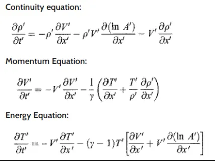
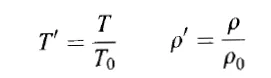
These are non-conservational forms of the governing equation and in dimensionless form, many cases of CFD dimensioned form of equations are used and they help provide a physical sense to the solution and ease of comparison, contrary to the dimensionless form used in case of this problem. The flow variables are expressed in terms of their reservoir counterpart with them. These variables range from 0 to 1.

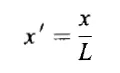
L denotes the length of the nozzle, we define a dimensionless length as,

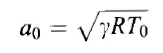
Denoting the speed of sound in the reservoir as ao, where

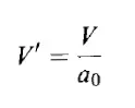
we define a dimensionless velocity as,

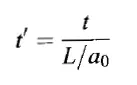
Also, the quantity Liao has the dimension of time, and we define a dimensionless time as

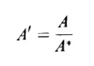
Finally, we ratio the local area A to the sonic throat area A* and define a dimensionless area as

Discretization of Equation

A different scheme is chosen that will allow for the most convenient and efficient time marching solution for Quasi-1-D nozzle flow, MacCormack's explicit technique for the numerical solution is used for the same reason.

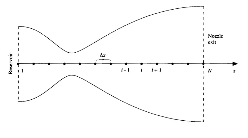
We divide the x-axis along with the nozzle into several discrete grid points; the first grid point, labelled point I, is assumed to be in the reservoir. Point ‘i’ is simply an arbitrary grid point, with points ‘i - 1’ and ‘i + 1’ as the adjacent points.

MacCormack's technique is a predictor-corrector method. In the time-marching approach, remember that we know the flow-field variables at time t, and we use the differential equations to solve explicitly for the variables at time t + Δt.

First, consider the predictor step. we set up the spatial derivatives as forwarding differences. Also, to reduce the complexity of the notation, we will drop the use of the prime to denote a dimensionless variable. In what follows, all variables are the non-dimensional variables, denoted earlier by the prime notation.

This being an explicit method, we find the time derivative by using previous state values and update the flow state variables. Then we proceed with the corrector step, these updated values are used and a backward difference scheme is used for the space derivatives. Then we take an average of the 2 calculated time derivatives for each flow field variable.

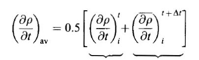
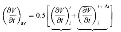
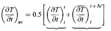
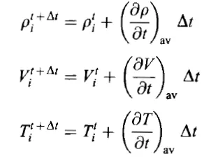
With these average values of time derivatives, we find the corrected values of flow field variables at time t + dt.

Calculator of Time Step

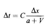
The governing system of equations is hyperbolic concerning time. A stability constraint that exists in this system is analogous. Calculating this time step at all grid points, i = 1 to i = N, by taking C = 0.5, and the minimum value amongst them is chosen, which is used to calculate the flow field variables.

Nozzle Shape and initial conditions

The nozzle shape, A = A(x), is specified and held fixed, independent of time, For the case illustrated in this section, we choose a parabolic area distribution given by

Therefore, in our choice of initial conditions, we have used any knowledge we may have about a given problem to intelligently pick some initial conditions so that they are chosen close to steady-state value so that there is no chance for the solution to go unstable. We are aware that the ‘T’ decreases and ‘V’ increases as the flow expands through the nozzle. This is exactly why initial conditions are chosen such that they qualitatively behave in the same way. For the convenience of the calculations, we assume the flow field variables, as a function of ‘x’.

Initial conditions at time t = 0,

ρ = 1-(0.3146*x)

T = 1-(0.2314*x)

V = [0.1 + (1.09)*x]*T^ 1/2

Boundary Conditions

Another aspect of the numerical solution is that of boundary conditions- an all-important aspect, because, without the physically proper implementation of boundary conditions and their numerically proper representation, we have no hope whatsoever in obtaining a proper numerical solution to our flow problem.

Subsonic inflow boundary (point1) :

Here, we must allow one variable to float. We choose the velocity V1, because on a physical basis we know the mass flow through the nozzle must be allowed to adjust the proper steady-state, and allowing V1 to float makes the most sense as part of this adjustment. The value of V1 changes with time and is calculated from information provided by the flow-field solutions over the internal points. We use linear extrapolation from points 2 and 3 to calculate V1 and we take rho (1) =1 and T(1) +1 as fixed values.

V(1) = 2* V(2) - V(3)

Supersonic outflow boundary (point N)

Here, we must allow all flow-field variables to float. We again choose to use linear extrapolation based on the flow field values at the internal points. Specifically, we have, for the non-dimensional variables.

VN = 2V(N-1) - V(N-2)

ρN = 2ρ(N-1) - ρ(N-2)

TN = 2T(N-1) - T(N-2)

Conservative Form

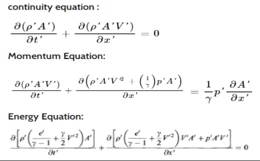
The conservative form of governing equations is represented in non-dimensional form, but this is to be converted to generic form.

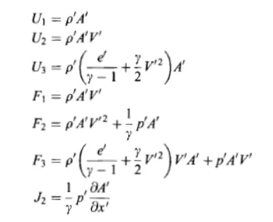
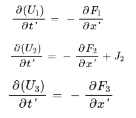
Now Substituting the LHS in the governing equations.

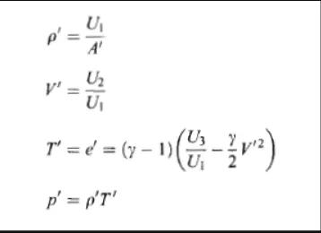
Once the Solution values (solution matrix of U) are calculated we can find the flow field variables (T, P, V, ρ).

‘F’ is the flux (Flux vector) F1, F2, F3 being the flux elements and J being the source term, using the above solution the flow field variables or the primitive variables are found (in Non-dimensional form). But it has a tendency to make the solution unstable, for which we express them as solution elements for each grid point.

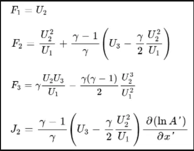
Now to solve the system we must discretize the equations MacCormack technique is used on the source and flux terms.

Predictor Step

To start we will first use initial conditions for U1, U2, U3 to determine the initial values of F1, F2, F3, and these values are used to calculate U1, U2, U3 in the next time steps in return. Forward differencing is applied in the predictor step first on the RHS and solving these gives the predicted values of the solution matrix elements.

Corrector step

These predicted values of the solution matrix element are used to determine the elements of the flux matrix. And the differentials are discretized in a backward fashion.

The time derivative of the elements of the solution matrix obtained from both the steps are taken and a mean is calculated for both;

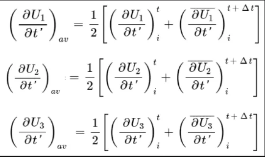
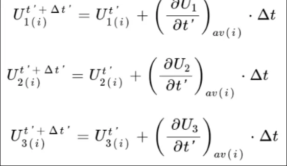
This process is repeated at every node for all time steps except at the boundary of the solution as we already know the results there. Using this we find our variables at the next time step as well.

For getting the initial conditions for the elements of the solution matrix ‘U’ we assume the variation of ρ’ and T’ as a function of ‘x’.

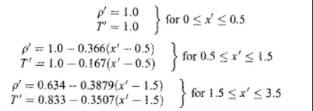
The variations here are slightly more accurate or realistic than the ones assume in the Non-conservative form initial condition and Shape of the nozzle, this is done so that the stability behaviour of the conservative form of governing equations becomes slightly more sensitive, which allows us to further improve and modify the initial conditions compared to the non-conservative form.

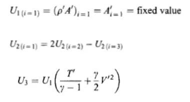
Boundary conditions: Subsonic Inflow boundary (point 1)

At this stage 2 of the flow field properties are considered fixed and only one is allowed to float the T’ and ρ’ fixed and equal to unity and the V’ is allowed to float.

Supersonic Outflow boundary (point N)

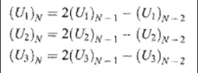
At the outflow boundary, all the flow field properties are allowed to float. The flow properties at a downstream, Supersonic outflow boundary are obtained by linear extrapolation from the 2 adjacent internal points.

Code

%% Non Conservative form
function [x,dt,rho,v,T,p,Mach,flow_rate,nt_grid,n_iter_n] = Non_Conservative_nozzle_flow(L,n,C,dx,nt,gama)
%% Initial condition of the nozzle flow
% input
x = linspace(0,L,n);
rho = 1-0.3146*x;
T = 1-0.2314*x;
v = (0.1+1.09*x).*T.^0.5;
A = 1+2.2*(x-1.5).^2;
Throat = (n+1)/2;          % Nodes across throat
nt_grid = 1:nt;            % 1400 Grid points equally spaced
initial_flow = rho.*v.*A;  % 'V' is allowed to float at point 1
Old_flow_rate = 0;         % reservoir area is large so flow rate is taken 0
%% Iterations
tolnce = 1e-4;             % Tolerance
error = 1000;              % error for tolerance comparison
n_iter_n = 1;
% Analytical Mass flow rate
Ana_m = 0.579*ones(n,n);
% Calculating minimum of dt calculated at all nodes
for m = 1:n
    dt_node(m) = C*(dx/(T(m)^(0.5) + v(m)));
end
% Time step
dt = min(dt_node);

%% MacCormack Technique
for i = 1:nt
    
    rho_old = rho;
    T_old = T;
    v_old = v;
    % First calculating the derivatives for the internal grid points for
    % each time step in the predictor step
    for z = 2:n-1
        dvdx = (v(z+1)-v(z))/dx;
        drhodx = (rho(z+1)-rho(z))/dx;
        dTdx = (T(z+1)-T(z))/dx;
        dlogAdx = (log(A(z+1))-log(A(z)))/dx;
        
        %% Governing Equation
        % Continuity Equation
        drhodt_p(z) = -rho(z)*dvdx - rho(z)*v(z)*dlogAdx - v(z)*drhodx;
        % Momentum Equation
        dvdt_p(z) = -v(z)*dvdx - (1/gama)*(dTdx + (T(z)/rho(z))*drhodx);
        % Energy Equation
        dTdt_p(z) = -v(z)*dTdx - (gama-1)*T(z)*(dvdx + (v(z)*dlogAdx));
        
        % Updating the solution of the predictor
        rho(z) = rho(z) + drhodt_p(z)*dt;
        v(z) = v(z) + dvdt_p(z)*dt;
        T(z) = T(z) + dTdt_p(z)*dt;
    end
    % Corrector step
    % Same values are calculeted for corrector step only backward in space
    for z = 2:n-1
        dvdx = (v(z)-v(z-1))/dx;
        drhodx = (rho(z)-rho(z-1))/dx;
        dTdx = (T(z)-T(z-1))/dx;
        dlogAdx = (log(A(z))-log(A(z-1)))/dx;
        
        %% Governing Equation
        % Continuity Equation
        drhodt_C(z) = -rho(z)*dvdx - rho(z)*v(z)*dlogAdx - v(z)*drhodx;
        % Momentum Equation
        dvdt_C(z) = -v(z)*dvdx - (1/gama)*(dTdx + (T(z)/rho(z))*drhodx);
        % Energy Equation
        dTdt_C(z) = -v(z)*dTdx - (gama-1)*T(z)*(dvdx + (v(z)*dlogAdx));        
    end
    % Finally taking the avrage of the time derivatives
    drhodt = 0.5*(drhodt_p + drhodt_C);
    dvdt = 0.5*(dvdt_p + dvdt_C);
    dTdt = 0.5*(dTdt_p + dTdt_C);
    
    % Final Step Update
    for z = 2:n-1
        rho(z) = rho_old(z) + drhodt(z)*dt;
        v(z) = v_old(z) + dvdt(z)*dt;
        T(z) = T_old(z) + dTdt(z)*dt;
    end
    % inlet Boundry Condition
    v(1) = 2*v(2) - v(3);
    % outlet boundry condition
    rho(n) = 2*rho(n-1) - rho(n-2);
    v(n) = 2*v(n-1) - v(n-2);
    T(n) = 2*T(n-1) - T(n-2);
    
    % Flow field variables of x
    p = rho.*T;    % pressure
    Mach = (v./((T).^0.5));
    flow_rate = rho.*v.*A;
    
    % Throat 
    T_throat(i) = T(Throat);
    p_throat(i) = p(Throat);
    rho_throat(i) = rho(Throat);
    Mach_throat(i) = Mach(Throat);
    v_throat(i) = v(Throat);
    flow_rate_throat(i) = flow_rate(Throat);
    
    error = max(abs(flow_rate-Old_flow_rate));
    if error > tolnce
        n_iter_n = n_iter_n + 1;
        Old_flow_rate = flow_rate;
    end
   figure(1)
   % Dimentionless flow field variables across nozzle at progressing time
   % step compared with analytical mass flow rate
   if i == 50
       plot(x, flow_rate, 'Linewidth',2);
       hold on
   else if i == 100
           plot(x, flow_rate, 'Linewidth',2);
           hold on
       else if i == 200
               plot(x, flow_rate, 'Linewidth',2);
               hold on
           else if i == 500
                   plot(x, flow_rate, 'Linewidth',2);
                   hold on
               else if i == 700
                       plot(x, flow_rate, 'Linewidth',2);
                       hold on 
                       plot(x, Ana_m, ':')
                       hold on
                       plot(x,initial_flow,'--')
                       
                       legend('50Delta','100Delta','200Delta','500Delta','700Delta','Analytical Solution','Initial Flow Rate');
                       title('Fluid Flow Through a Nozzle at Progressing Time Before Steady State - Nonconservative Form (Dimensionless)');
                       xlabel('Dimensionless x/L','Fontsize', 12);
                       ylabel('Nonconservative Mass flow rate', 'Fontsize', 12);
                   end
               end
           end
       end
   end
end

% Flow field variables at each time nodes in there steady state
figure(2)
sgtitle(sprintf('Flow variables steady state variables (nonconservative form), number of time steps = %d', i))
subplot(5,1,1)
plot(x,Mach,'g','Linewidth',3);
xlabel('Dimensionless Length');
ylabel('Mach-Number');
legend('Mach Number')

subplot(5,1,2)
plot(x,v,'b','Linewidth',3);
xlabel('Dimensionless Velocity');
ylabel('V/a_knot');
legend('Dimensionless Velocity')

subplot(5,1,3)
plot(x,rho,'k','Linewidth',3);
xlabel('Dimensionless Density');
ylabel('rho/rho_knot');
legend('Dimensionless Density')

subplot(5,1,4)
plot(x,T,'y','Linewidth',3);
xlabel('Dimensionless Temprature');
ylabel('T/T_knot');
legend('Dimensionless Temprature')

subplot(5,1,5)
plot(x,p,'r','Linewidth',3);
xlabel('Dimensionless Pressure');
ylabel('p/p_knot');
legend('Dimensionless Pressure')

figure(3)
% Time marching solution of the flow field variables at the throat
plot(nt_grid,T_throat,'Linewidth',2)
hold on
plot(nt_grid,p_throat,'Linewidth',2)
hold on
plot(nt_grid,rho_throat,'Linewidth',2)
hold on
plot(nt_grid,Mach_throat,'Linewidth',2)
hold on
plot(nt_grid,v_throat,'Linewidth',2)
hold on
plot(nt_grid,flow_rate_throat,'Linewidth',2)

legend('Dimensionless Temprature(T/T_knot)','Dimensionless Pressure(P/P_knot)','Dimensionless Density(rho/rho_knot)','Mach Number','Dimensionless Velocity(V/a_knot)','Flow Rate')
xlabel('Number of Time Steps')
ylabel('Non-dimensional Flow field variables')
title('Progression of Flow field variables at throat in nonconservative form')
end

%% Conservative form

function [dt,rho,T,p,Mach,flow_rate_c,Ana_m,n_iter_c,tlrnce] = Conservative_nozzle_flow(L,n,C,dx,gama,nt)
%% Initial condition of nozzle flow
% Input
x = linspace(0,L,n);
A = 1 + 2.2*(x-1.5).^2;
Throat = (n +1)/2;
nt_grid = 1:nt;
% Analalytical mass flow rate
Ana_m = 0.579*ones(n,n);
n_iter_c = 1;
% initial mass flow rate
U2_i = 0.59;
Old_flow_rate = 0;
tlrnce = 1e-4;
error = 1000;
%% Computation
% Floating value of density and temprature
for i = 1:n
    if x(i) >= 0 && x(i) <= 0.5
        rho(i) = 1.0;
        T(i) = 1.0;
    else if x(i) >= 0.5 && x(i) <= 1.5
            rho(i) = 1 - (0.366*(x(i) - 0.5));
            T(i) = 1 - (0.167*(x(i)-0.5));
        else if x(i) >= 1.5 && x(i) <= 3
                rho(i) = 0.634 - (0.3879*(x(i) - 1.5));
                T(i) = 0.833 - (0.3507*(x(i) - 1.5));
            end
        end
    end
end

% Computation of solution vector
for j = 1:n
    v(j) = U2_i/(rho(j)*A(j));
    U1(j) = rho(j)*A(j);
    U2(j) = rho(j)*A(j)*v(j);
    U3(j) = rho(j)*A(j)*((T(j)/(gama-1)) + (0.5*gama*v(j)^2));
end

% Minimum magnitude of time step dt
for k = 1:n
    dt_x(k) = C*(dx/(T(k)^(0.5) + v(k)));
end

% Time step
dt = min(dt_x);

U2_initial = U2;

for q = 1:nt
    
    U1_old = U1;
    U2_old = U2;
    U3_old = U3;
    
    % Flux matrix as a functio of solution matrix
    F1 = U2;
    F2 = ((U2.^2)./(U1)) + (((gama - 1)/gama).*(U3 - ((gama/2).*(((U2.^2)./U1)))));
    F3 = ((gama.*U2.*U3)./U1) - (gama.*(gama-1)/2)*((U2.^3)./U1.^2);
    
    % Space iterrations on internal nodes
    % Pridictor Steps
    for i = 2:n-1
        dF1dx = (F1(i+1) - F1(i))/dx;
        dF2dx = (F2(i+1) - F2(i))/dx;
        dF3dx = (F3(i+1) - F3(i))/dx;
        
        %% Governing equation
        % Continuity equation 
        dU1dt_p(i) = -dF1dx;
        
        % Momentum equation
        J2(i) = ((1/gama)*rho(i)*T(i)*((A(i+1) - A(i))/dx));     % Source term
        dU2dt_p(i) = -dF2dx + J2(i);
        
        % Energy equation
        dU3dt_p(i) = -dF3dx;
        
        % Updating Solution vector
        U1(i) = U1(i) + dU1dt_p(i)*dt;
        U2(i) = U2(i) + dU2dt_p(i)*dt;
        U3(i) = U3(i) + dU3dt_p(i)*dt;
    end
    
    % Updating the initial value
    rho = U1./A;
    v = U2./U1;
    T = (gama -1).*((U3./U1)-(0.5*gama.*v.^2));
    p = rho.*T;
    % Computing flux matrix using values from pridicted values
    F1 = U2;
    F2 = ((U2.^2)./(U1)) + (((gama - 1)/gama).*(U3 - ((gama/2).*(((U2.^2)./U1)))));
    F3 = ((gama.*U2.*U3)./U1) - (gama.*(gama-1)/2)*((U2.^3)./U1.^2);
    
    % Corrector Step
    for j = 2:n-1
        dF1dx = (F1(j) - F1(j-1))/dx;
        dF2dx = (F2(j) - F2(j-1))/dx;
        dF3dx = (F3(j) - F3(j-1))/dx;
        
        %% Governing Equation
        % Continuity Equation
        dU1dt_c(j) = -dF1dx;
        
        % Momentum Equation
        J2(j) = ((1/gama)*rho(j)*T(j)*((A(j)-A(j-1))/dx));
        dU2dt_c(j) = -dF2dx + J2(j);
        
        % Energy Equation
        dU3dt_c(j) = -dF3dx;
        
    end
    
    % Avrage of time derivatives
    dU1dt = 0.5*(dU1dt_p + dU1dt_c);
    dU2dt = 0.5*(dU2dt_p + dU2dt_c);
    dU3dt = 0.5*(dU3dt_p + dU3dt_c);
    
    % Final computation
    for k = 2:n-1
        U1(k) = U1_old(k) + dU1dt(k)*dt;
        U2(k) = U2_old(k) + dU2dt(k)*dt;
        U3(k) = U3_old(k) + dU3dt(k)*dt;
    end
    
    % inlet Boundary Condition
    U1(1) = rho(1)*A(1);
    U2(1) = 2*U2(2) - U2(3);
    v(1) = U2(1)/(rho(1)*A(1));
    U3(1) = U1(1)*((T(1)/(gama - 1))+((gama*0.5)*v(1)^2));
    
    % Outlet Condition
    U1(n) = 2*U1(n-1) - U1(n-2);
    U2(n) = 2*U2(n-1) - U2(n-2);
    U3(n) = 2*U3(n-1) - U3(n-2);
    
    % Update of primary variable
    rho = U1./A;
    v = U2./U1;
    T = (gama - 1).*((U3./U1) - (0.5*gama.*v.^2));
    
    % Calculetion of other flow field variable
    p = rho.*T;
    Mach = (v./((T).^0.5));
    flow_rate_c = rho.*v.*A;
    
    % Computation of flow field values at the throat
    rho_throat(q) = rho(Throat);
    v_throat(q) = v(Throat);
    T_throat(q) = T(Throat);
    p_throat(q) = p(Throat);
    Mach_throat(q) = Mach(Throat);
    flow_rate_throat(q) = flow_rate_c(Throat);
    
    error = max(abs(flow_rate_c - Old_flow_rate));
    if error > tlrnce
        n_iter_c = n_iter_c + 1;
        Old_flow_rate = flow_rate_c;
    end
    % Dimensionless Mass flow rate across nozzle at varing time step
    % compared with analytical mass flow rate
    %% Plotting of results
    figure(4)
    if q == 50
        plot(x,flow_rate_c,'Linewidth',2)
        hold on
    else if q == 100
            plot(x,flow_rate_c,'Linewidth',2)
            hold on
        else if q == 200
                plot(x,flow_rate_c,'Linewidth',2)
                hold on
            else if q == 500
                    plot(x,flow_rate_c,'Linewidth',2)
                    hold on
                else if q == 700
                        plot(x,flow_rate_c,'Linewidth',2)
                        hold on
                        plot(x,Ana_m,':')
                        hold on
                        plot(x,U2_initial,'--')
                        
                        legend('50 Delta','100 Delta','200 Delta','500 Delta','700 Delta','Analytical Solution','Initial Flow Rate');
                        title('Dimensionless Mass flow rate across the nozzle progressing in time in Conservative form');
                        xlabel('Dimensionless Length x/L','Fontsize',10);
                        ylabel('Mass Flow Rate Conservative','Fontsize', 11)
                        axis([0 3 0.5 1])
                    end
                end
            end
        end
    end
end
% Ploting Steady State value of flow field variable ant each node
figure(5)
sgtitle(sprintf('Steady State value of the flow field variables in conservative form, number of time steps = %d',q))
subplot(5,1,1)
plot(x,Mach,'b','Linewidth',2)
xlabel('Dimensionless Length');
ylabel('Mach Number');
legend('Mach Number')

subplot(5,1,2)
plot(x,v,'k','Linewidth',2)
xlabel('Dimensionless Velocity');
ylabel('V/a_knot');
legend('Dimensionless Velocity')

subplot(5,1,3)
plot(x,rho,'y','Linewidth',2)
xlabel('Dimensionless Density');
ylabel('Rho/Rho_knot');
legend('Dimensionless Density')

subplot(5,1,4)
plot(x,T,'r','Linewidth',2)
xlabel('Dimensionless Temprature');
ylabel('T/T_knot');
legend('Dimensionless Temprature')

subplot(5,1,5)
plot(x,p,'g','Linewidth',2)
xlabel('Dimensionless Pressure');
ylabel('p/p_knot');
legend('Dimensionless Pressure')

% Flow field Variables at the nozzle throat
figure(6)
plot(nt_grid,Mach_throat,'Linewidth',2)
hold on
plot(nt_grid,rho_throat,'Linewidth',2)
hold on
plot(nt_grid,v_throat,'Linewidth',2)
hold on
plot(nt_grid,T_throat,'Linewidth',2)
hold on
plot(nt_grid,p_throat,'Linewidth',2)

legend('Mach Number','Dimensionless density (rho/rho_knot)','Dimensionless Velocity(V/a_knot)','Dimensionless Temprature (T/T_knot)','Dimensionless Pressure (p/p_knot)')
xlabel('Progression of time');
axis([0 1400 0.5 1.2])
title('Conservative form of variation of flow field variable')

end

%% Compiletion

clear all
close all
clc

%% Inputs
L = 3;
n = 31;
dx = L/(n-1);
C = 0.5;
nt = 1400;
gama = 1.4;

%% Computation
% Non-Conservative form
tic
[x,dt,rho,v,T,p,Mach,flow_rate_n,nt_grid,n_iter_n] = Non_Conservative_nozzle_flow(L,n,C,dx,nt,gama);
toc
time_non_conservative = toc;
fprintf('Time of exicuting for non-conservative form = %0.4gs',time_non_conservative)

% Solving Governing equation in conservative form
tic
[dt,rho,T,p,Mach,flow_rate_c,Ana_m,n_iter_c,tlrnce] = Conservative_nozzle_flow(L,n,C,dx,gama,nt);
toc
Time_conservative = toc;
fprintf('Time of exicution of conservative form = %0.4gs',Time_conservative)

figure(7)
plot(x,flow_rate_n,'Linewidth',2)
hold on
plot(x,flow_rate_c,'LInewidth',2)
hold on
plot(x,Ana_m,'Linewidth',2)
legend('Nonconservative form','Conservative Form','Analytical Solution')
xlabel('Dimensionless length x/L','Fontsize',10);
ylabel('Dimensionless mass flow rate in Non Conservative form','Fontsize',10);
title(sprintf(['comparision of steady state mass flow variation (on magnified scale) obtained with nonconservative and conservative form of the governing flow equations']))

% Using bar graph to compare the convergence rate
figure(8)
no_of_iter = [n_iter_n n_iter_c];
bar(no_of_iter)

set(gca,'xticklabel',{'Non Conservative Form','Conservative Form'});
ylabel('No. of iterations');
title(sprintf(['Number of iterations to attain steady state for a tolerance of %g'],tlrnce));
legend('Number of iterations')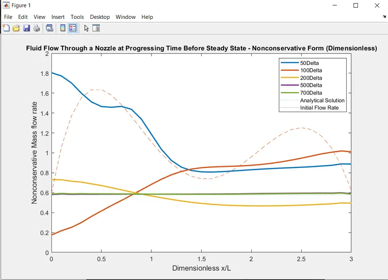

This is a non-dimensional mass flow rate distribution across the nozzle at a progressing timestep in Non-conservative form.

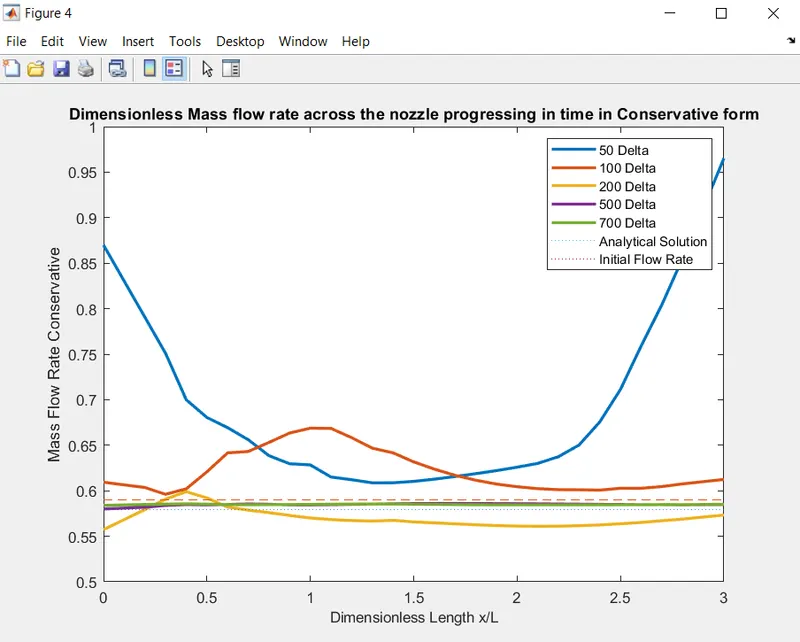
This is a non-dimensional mass flow rate distribution across the nozzle at a progressing timestep in conservative form.

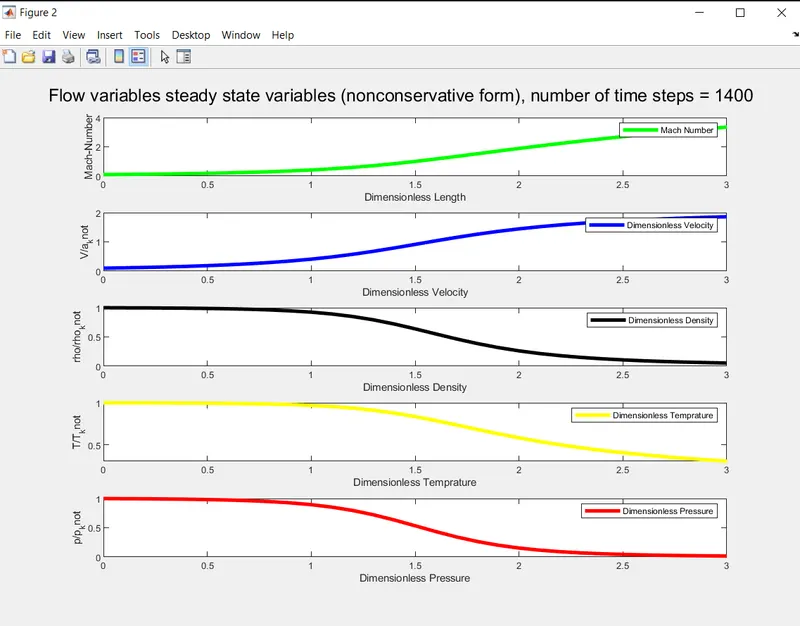
Steady state values of flow field variables in nonconservative form. Which are in Dimensionless form.

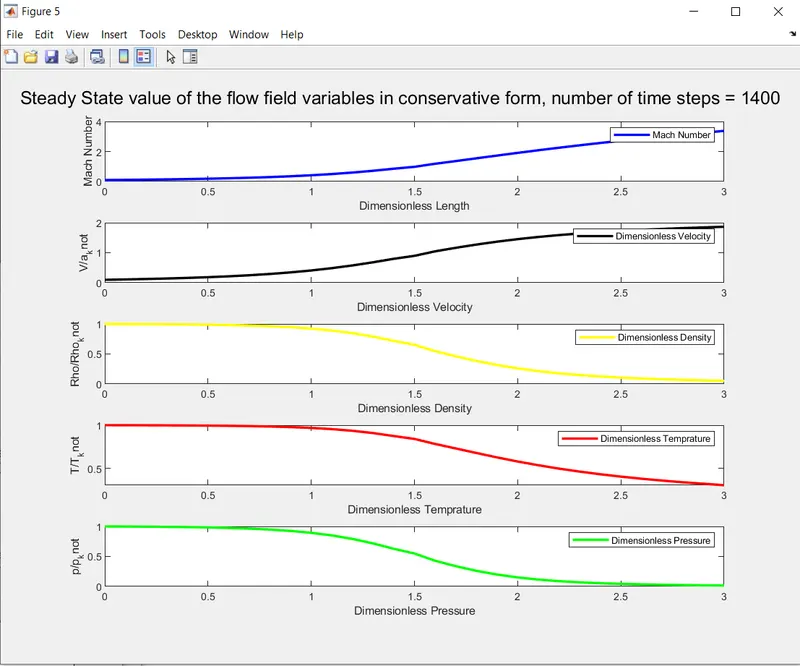
Steady state values of flow field variables in conservative form. And are the dimensionless form of the variables.

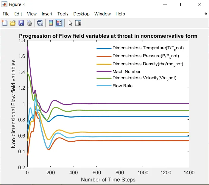
Dimensionless flow field variables’ progression through the nozzle throat in the non-conservative form attaining steady state over the course of progression. The oscillations stabilize at around 400 timesteps.

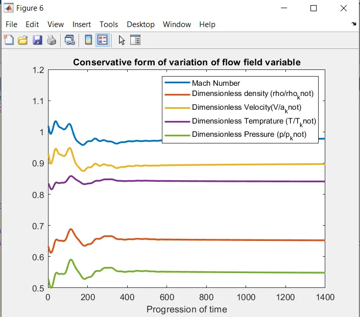
Dimensionless flow field variables’ progression through the nozzle throat in the conservative form attaining steady state over the course of progression. The oscillations stabilize at around 500 timesteps.

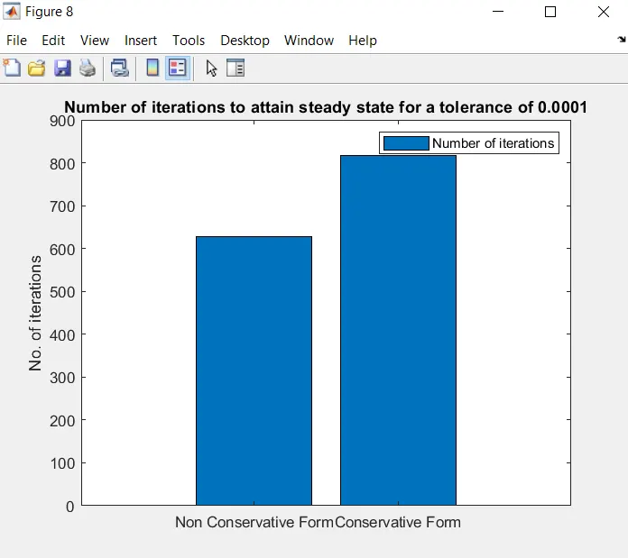
Comparison of the 2 forms of the nozzle flow time-step. For the tolerance of 1e-4. This plot proves the the nonconservative form is faster than the conservative form

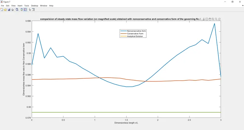
This is the comparison of the steady state mass flow rate obtained from both conservative and non conservative forms of governing equations.

The conservative form preserves the mass flow throughout the flow field, mainly because it is a dependent variable and a primary result from these equations. And the non conservative form of the equations are the primitive flow field variables, and the mass flow rate is the secondary result.

And finally we can conclude that a clear priority is given to the conservative forms of the governing equation over the non conservative form.

1. The conservation form yields a better mass flow distribution. The conservation form simply does a better job of conserving mass since the mass flow itself is a dependent value.
2. There is no clear superiority of either form in terms of accuracy of result. The nonconservation form seems to produce slightly more accurate results for the primitive variables, and the conservation form seems to produce slightly more accurate results for the flux variables. The results in either case are certainly satisfactory.
3. Comparing the amount of calculation effort to achieve a solution, we note that the solution of the conservation form requires marginally more work. Most of this due to the need to decode the primitive variables from the flux variables. Such decoding is not necessary when solving nonconservative forms.
4. Non conservative form attains steady state faster than the conservative form.
5. Both the forms don't rely on the grid.

Report Doc: https://docs.google.com/document/d/1ZMuQ4D32EpkJsZfuBXEp4-Fgfk0W0_cAtKPJE0XH8TY/edit?usp=sharing