Introduction

Thermal conduction is the transfer of internal energy by microscopic collisions of particles and the movement of electrons within a body. The collision leads to the transfer of the internal energy whether it be Kinetic energy or Potential Energy.

The 2D Heat equation ∂T/∂t -∝(∂2T/∂x2 + ∂2T/∂y2) = 0 is an elliptical equation, which means the information is propagated everywhere. Change in properties is affected by every point around it and affects every point around it in return.

The elliptical equation is solved for a closed domain with boundaries at all sides.

For Steady State conduction:

A form of conduction that happens when the temperature difference driving the conduction is constant so that the spatial distribution of temperatures in the conducting object does not change any further. So the spatial temperature derivative is constant and the time-temperature derivative is zero.

(∂2T/∂x2 + ∂2T/∂y2) = 0

For Unsteady State conduction:

A form of conduction in which the time-dependent temperature derivative is non zero and affects the overall temperature and the conduction in a system, and temperature changes in time toward a new equilibrium. It can be considered that new sources and sinks are suddenly introduced in a pre-existing system at the boundaries. As the equilibrium is attained the system returns to the original condition and the Heat energy remains conserved.

∂T/∂t -∝(∂2T/∂x2 + ∂2T/∂y2) = 0

Problem Question

To solve the steady and unsteady 2D heat conduction equation and then plotting the results as a contour graph.

Assuming the equal number of grid points/nodes in the x and y-axis [nx = ny].

The boundary conditions given are;

Top Boundary temperature = 600 K,

Bottom Boundary temperature = 900 K,

Left Boundary temperature = 400 K,

Right Boundary temperature = 800 K,

The initial temperature within the domain is assumed to be 300 K uniformly,

Solution

The Given question is to be solved under different conditions

1. States: Steady-state & Unsteady state condition,
2. Methods to be used in unsteady-state: Implicit and Explicit,
3. Schemes: Jacobi, Gauss-Seidel & Successive over Relaxation,

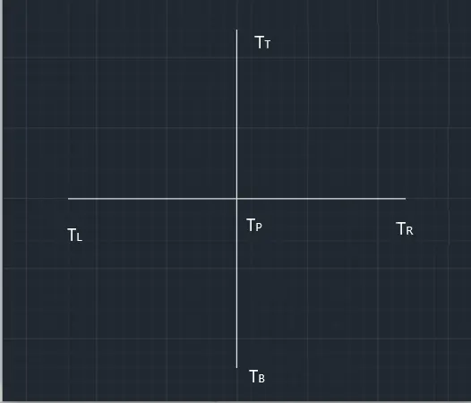
Dist form TL to TP = TP to TR = x, TT to TP = TP to TB = y

TL= Left Boundary [T(i-1, j)]

TP = Point of concern [T(i, j)]

TR = Right Boundary [T(i+1, j)]

TT = Top Boundary [T(i, j+1)]

TB = Bottom Boundary [T(i, j-1)]

Steady State Condition

A fluid state in which there are no changes in fluid properties concerning time is known as a steady-state. The energy remains conserved.

(∂2T/∂x2 + ∂2T/∂y2) = 0

∂T/∂t = 0

Using the central differencing scheme

(TL - 2* TP + TR)/△x2 + ( TT- 2*TP + TB )/△y2 = 0

Simplifying the given equation;

Jacobi Method,

2* TP ((1/△x2) + (1/△y2)) =( (TL + TR)/△x2) + ( ( TT + TB )/△y2)

k = 2*[(1/△x2) + (1/△y2)]

Tn+1P = (1/k) * ( (TL + TR)/△x2) + ( ( TT + TB )/△y2)n

%% Jacobi iterative solver for Steady State 

function [out] = jacobi_steady(nx, ny, X, Y, dx, dy,T_old, T, tolerance, error, k)
% Jacobi method for steady state
Jac_iter = 1;
tic
while(error > tolerance)
    for i = 2:nx-1
        for j = 2:ny-1
            term1 = (T_old(i-1, j) + T_old(i+1, j))/(k*(dx^2));
            term2 = (T_old(i, j-1) + T_old(i, j+1))/(k*(dy^2));
            T(i,j) = term1 + term2;
        end
    end
    error = max(max(abs(T_old - T)));
    T_old = T;
    Jac_iter = Jac_iter + 1;
end
iter_time = toc;

figure(1)
[a,b] = contourf(X, Y, T);
set(gca,'YDIR','reverse');
colormap(jet)
clabel(a,b)
xlabel('X Length Domain');
ylabel('Y Length Domain');
txt1 = sprintf('Jacobi Method Iteration = %d', Jac_iter);
txt2 = sprintf('Jacobi Method Simulation Time = %f s', iter_time);
txt3 = sprintf('Final Error = %f', error);
colorbar
title({'Steady State';txt1;txt2;txt3});

out = iter_time;
end

-------------------------------------------------------------------------------------------------------------------------------------------

Gauss-Seidel method is similar, the only difference is that as the points on the grid are getting computed they are fed into the iterative solver to compute the next grid point for the generation which is being computed.

Tn+1P = (1/k) * ( (TL + TR)/△x2) + ( ( TT + TB )/△y2)n + 1

%% Gauss-Seidel Solver for steady-state

function [out] = gauss_seidel_steady(nx, ny, X, Y, dx, dy,T_old, T, tolerance, error, k)
% Gauss Seidel method for steady state
gs_iter = 1;

tic
while(error > tolerance)
    for i = 2:nx-1
        for j = 2:ny-1
            term1 = (T(i-1, j) + T_old(i+1, j))/(k*(dx^2));
            term2 = (T(i, j-1) + T_old(i, j+1))/(k*(dy^2));
            T(i,j) = term1 + term2;
        end
    end
    error = max(max(abs(T_old - T)));
    T_old = T;
    gs_iter = gs_iter + 1;
end
iter_time = toc;

figure(2)
[a,b] = contourf(X, Y, T);
colormap(jet)
clabel(a,b)
xlabel('X Length Domain');
ylabel('Y Length Domain');
txt1 = sprintf('Gauss Seidel Method Iteration = %d', gs_iter);
txt2 = sprintf('Gauss Seidel Method Simulesion Time = %f s', iter_time);
txt3 = sprintf('Final Error = %f', error);
colorbar
title({'Steady State';txt1;txt2;txt3});
set(gca,'YDIR','reverse')
out = iter_time;
end

-------------------------------------------------------------------------------------------------------------------------------------------

Successive Over-relaxation is a variant of the Jacobi and Gauss-Seidel method and using those solvers and with the help of the relaxation factor, it is computing the results and decreasing the number of iterations.

Tn+1P = (1 - w)*TnP w * ( (TL + TR)/△x2) + ( ( TT + TB )/△y2)n + 1

%% Successive Over-Relaxation method for steady-state

function [out] = sor_steady(nx, ny, x, y, dx, dy,T_old, T, tolerance, error, k)
% Successive Over-Relaxation method for steady state
sor_iter = 1;
w = 1.2;    % Over relaxation factor

tic
while(error > tolerance)
    for i = 2:nx-1
        for j = 2:ny-1
            term1 = (T(i-1, j) + T_old(i+1, j))/(k*(dx^2));
            term2 = (T(i, j-1) + T_old(i, j+1))/(k*(dy^2));
            T(i,j) = (1-w)*T_old(i,j) + (term1 + term2)*w;
        end
    end
    error = max(max(abs(T_old - T)));
    T_old = T;
    sor_iter = sor_iter + 1;
end
iter_time = toc;

figure(3)
[a,b] = contourf(x, y, T);
colormap(jet)
clabel(a,b)
xlabel('X Length Domain');
ylabel('Y Length Domain');
txt1 = sprintf('Successive Over-Relaxation Method Iteration = %d', sor_iter);
txt2 = sprintf('Successive Over-Relaxation Method Simulation Time = %f s', iter_time);
txt3 = sprintf('Final Error = %f', error);
colorbar
title({'Steady State';txt1;txt2;txt3});
set(gca,'YDIR','reverse')
out = iter_time;
end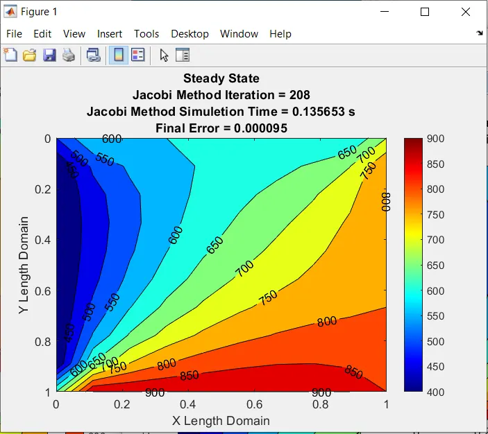

Jacobi Method for Steady State

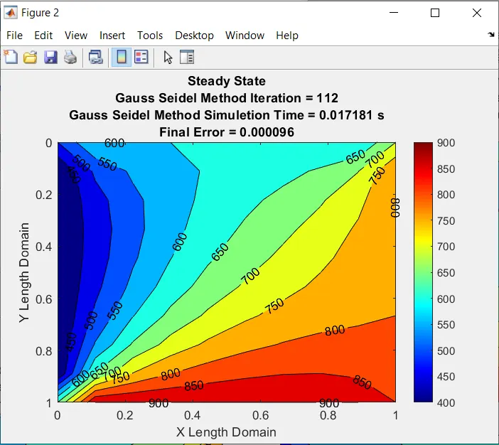
Gauss-Seidel Method for Steady State

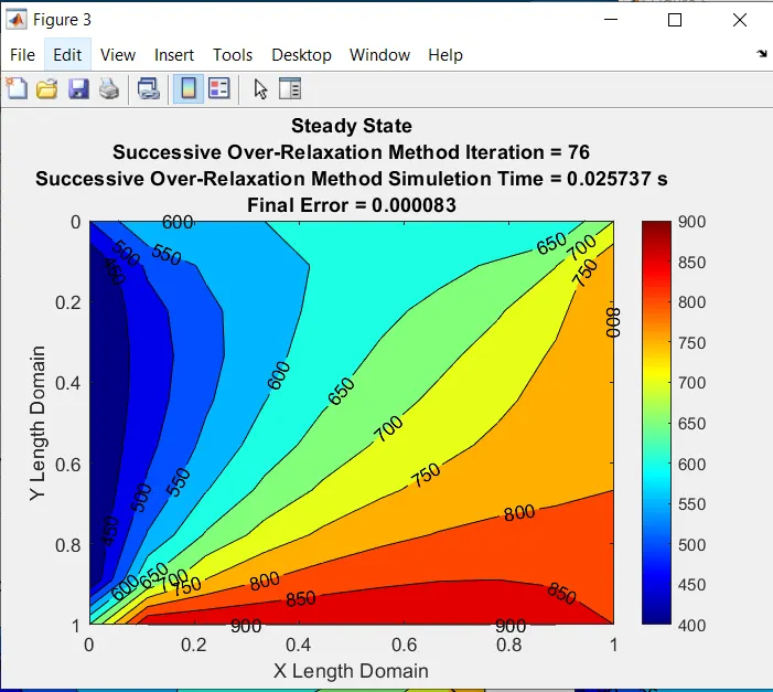
SOR method for steady-state

--------------------------------------------------------------------------------------------------------------------------------------------------------------------------------------------------------------------------------------------------------------------------------------

Transient State Condition

A fluid state in which there is a change in fluid properties concerning time is an unsteady state a.k.a. Transient State.

∂T/∂t -∝(∂2T/∂x2 + ∂2T/∂y2) = 0

Discretizing the equation we’ll use a forward differencing scheme for the time derivative and a backward differencing scheme for the spatial derivatives.

((TPn + 1 + TPn)/△t) - α[ (TL - 2* TP + TR)/△x2 + ( TT- 2*TP + TB )/△y2 ] = 0

K1 =α△t/△x2 K2 =α△t/△y2

TPn + 1 = TPn+ K1 (TL - 2* TP + TR) +K2 ( TT- 2*TP + TB )

Implicit Form

Solving the above equation to determine the implicit form of Jacobi Iterative solver,

TPn + 1 = [TPn+ K1 (TLn + TRn) +K2 ( TTn+ TBn ) ] / (1 + 2*K1 + 2*K2)

%% Transient-Implicit Condition Jacobi Iterative solver

function [out] = implicit_jacobi(nx, ny, x, y, T_old, T, t, dt, tolerance, error, k1, k2)
% Implicit Jacobi method for Transient state

nt = t/dt;
jac_iteration = 1;
Tpre = T;
tic
for m = 1:nt
        error=9e9;
    while(error > tolerance)
        for i = 2:nx-1
            for j = 2:ny-1
                term1 = (T_old(i-1, j) + T_old(i+1, j));
                term2 = (T_old(i, j-1) + T_old(i, j+1));
                T(i, j) = (Tpre(i, j) + (k1*term1) + (k2*term2))/(1 + 2*k1 + 2*k2);
            end
        end
        error = max(max(abs(T_old - T)));
        T_old = T;
        jac_iteration = jac_iteration + 1;
       
    end
    Tpre = T;
end
iteration_time = toc;
figure(4)
[a, b] = contourf(x, y, T);
colormap(jet)
clabel(a,b);
xlabel('X Length Domain');
ylabel('Y Length Domain');
txt1 = sprintf('Implicit Jacobi Method Iteration = %d', jac_iteration);
txt2 = sprintf('Implicit Jacobi Method Simulation Time = %f s', iteration_time);
txt3 = sprintf('Final Error = %f', error);
colorbar
title({'Transient State';txt1;txt2;txt3});
set(gca,'YDIR','reverse')
out = iteration_time;
end

-------------------------------------------------------------------------------------------------------------------------------------------

Solving the above equation to determine the implicit form of Gauss-Seidel Iterative solver,

TPn + 1 = [TPn+ K1 (TLn + 1 + TRn + 1) +K2 ( TTn + 1+ TBn + 1 ) ] / (1 + 2*K1 + 2*K2)

%% Transient-Implicit Gauss Seidel solver

function [out] = implicit_gauss_seidel(nx, ny, x, y, T_old, T, t, dt, tolerance, error, k1, k2)
% Implicit Gauss seidel method for Transient state

Tpre = T;
nt = t/dt;
gs_iteration = 1;

tic
for m = 1:nt
    error = 9e9;
    while(error > tolerance)
        for i = 2:nx-1
            for j = 2:ny-1
                term1 = T(i-1, j) + T_old(i+1, j);
                term2 = T(i, j-1) + T_old(i, j+1);
                T(i,j) = (Tpre(i,j) + (k1*term1) + (k2*term2))/(1 + 2*k1 + 2*k2);
            end
        end
        error = max(max(abs(T_old - T)));
        T_old = T;
        gs_iteration = gs_iteration + 1;
    end
    Tpre = T;
end
iter_time = toc;

figure(5)
[a, b] = contourf(x, y, T);
colormap(jet)
clabel(a, b);
xlabel('X Length Domain');
ylabel('Y Length Domain');
txt1 = sprintf('Implicit Gauss-Seidel Method Iteration = %d', gs_iteration);
txt2 = sprintf('Implicit Gauss-seidel Method Simuletion Time = %f s', iter_time);
txt3 = sprintf('Final Error = %f', error);
colorbar
title({'Transient State';txt1;txt2;txt3});
set(gca,'YDIR','reverse')
out = iter_time;
end

-------------------------------------------------------------------------------------------------------------------------------------------

Solving the above equation to determine the implicit form of Successive over-relaxation Iterative solver,

TPn + 1 =[[TPn+ K1 (TLn + 1 + TRn + 1) +K2 ( TTn + 1+ TBn + 1 ) ] / (1 + 2*K1 + 2*K2)]*w + (TPn)(1-w)

%% Transient-Implicit SOR solver

function [out] = implicit_sor(nx, ny, x, y, T_old, T, t, dt, tolerance, error, k1, k2)
% Implicit Successive Over-Relaxation method for Transient state

Tpre = T;
nt = t/dt;
sor_iteration = 1;
w = 1.1;                 % Over relaxation Factor

tic
for m = 1:nt
    error = 9e9;
    while(error > tolerance)
        for i = 2:nx-1
            for j = 2:ny-1
                term1 = T(i-1, j) + T_old(i+1, j);
                term2 = T(i, j-1) + T_old(i, j+1);
                T(i,j) = (1-w)*T_old(i,j) + (w*((Tpre(i,j) + (k1*term1) + (k2*term2))/(1 + 2*k1 + 2*k2)));
            end
        end
        error = max(max(abs(T_old - T)));
        T_old = T;
        sor_iteration = sor_iteration + 1;
    end
    Tpre = T;
end
iter_time = toc;

figure(6)
[a, b] = contourf(x, y, T);
colormap(jet)
clabel(a, b);
xlabel('X Length Domain');
ylabel('Y Length Domain');
txt1 = sprintf('Implicit Successive Over-Relaxation Method Iteration = %d', sor_iteration);
txt2 = sprintf('Implicit Successive Over-Relaxation Method Simulation Time = %f s', iter_time);
txt3 = sprintf('Final Error = %f', error);
colorbar
title({'Transient State';txt1;txt2;txt3});
set(gca,'YDIR','reverse')
out = iter_time;
end

We will be using these schemes to solve the successive over-relaxation, gauss seidel, and Jacobi iterative solvers for the Implicit condition.

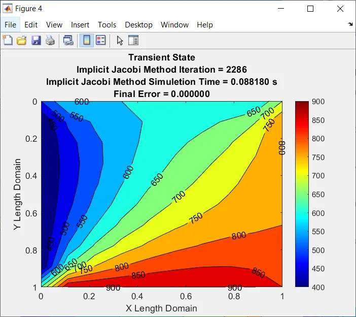
Implicit Jacobi Method

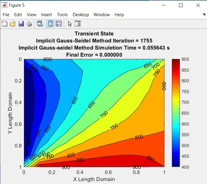
Implicit Gauss-Seidel Method

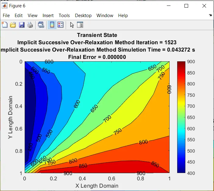
Implicit SOR Method

-------------------------------------------------------------------------------------------------------------------------------------------

Explicit Form

Solving the above equation to determine the explicit form of Jacobi Iterative solver,

TPn + 1 = [ (1 - 2*K1 - 2*K2)TPn+ K1 (TLn + TRn) +K2 ( TTn+ TBn ) ]

%% Transient-Explicit Jacobi Solver

function [out] = explicit_jacobi(nx, ny, x, y, T_old, T, t, dt, tolerance, error, k1, k2)
% Explicit Jacobi method for Transient state

Tpre = T;
nt = t/dt;
exp_jac_iter = 1;

tic
for m = 1:nt
    error = 9e9;
    while(error > tolerance)
        for i = 2:nx-1
            for j = 2:ny-1
                term1 = (T_old(i-1, j) + T_old(i+1, j));
                term2 = (T_old(i, j-1) + T_old(i, j+1));
                T(i,j) = (Tpre(i,j)*(1 - 2*k1 - 2*k2) + (k1*term1) + (k2*term2));
            end
        end
        error = max(max(abs(T_old - T)));
        T_old = T;
        exp_jac_iter = exp_jac_iter + 1;
    end
    Tpre = T;
end
iter_time = toc;

figure(7)
[a, b] = contourf(x, y, T);
colormap(jet)
clabel(a,b);
xlabel('X Length Domain');
ylabel('Y Length Domain');
txt1 = sprintf('Explicit Jacobi Method Iteration = %d', exp_jac_iter);
txt2 = sprintf('Explicit Jacobi Method Simuletion Time = %f s', iter_time);
txt3 = sprintf('Final Error = %f', error);
colorbar
title({'Transient State';txt1;txt2;txt3});
set(gca,'YDIR','reverse')
out = iter_time;
end

-------------------------------------------------------------------------------------------------------------------------------------------

Solving the above equation to determine the explicit form of Gauss-Seidel Conditions solver,

TPn + 1 = [ (1 - 2*K1 - 2*K2)TPn+ K1 (TLn + 1 + TRn + 1) +K2 ( TTn + 1+ TBn + 1 ) ]

%% Transient-Explicit Gauss-Seidel Solver

function [out] = explicit_gauss_seidel(nx, ny, x, y, T_old, T, t, dt, tolerance, error, k1, k2)
% Explicit Gauss seidel method for Transient state

Tpre = T;
nt = t/dt;
exp_gs_iter = 1;

tic
for m = 1:nt
    error = 9e9;
    while(error > tolerance)
        for i = 2:nx-1
            for j = 2:ny-1
                term1 = (T(i-1, j) + T_old(i+1, j));
                term2 = (T(i, j-1) + T_old(i, j+1));
                T(i,j) = (Tpre(i,j)*(1 - 2*k1 - 2*k2) + (k1*term1) + (k2*term2));
            end
        end
        error = max(max(abs(T_old - T)));
        T_old = T;
        exp_gs_iter = exp_gs_iter + 1;
    end
    Tpre = T;
end
iter_time = toc;

figure(8)
[a, b] = contourf(x, y, T);
colormap(jet)
clabel(a,b);
xlabel('X Length Domain');
ylabel('Y Length Domain');
txt1 = sprintf('Explicit Gauss Seidel Method Iteration = %d', exp_gs_iter);
txt2 = sprintf('Explicit Gauss Seidel Method Simulation Time = %f s', iter_time);
txt3 = sprintf('Final Error = %f', error);
colorbar
title({'Transient State';txt1;txt2;txt3});
set(gca,'YDIR','reverse')
out = iter_time;
end

-------------------------------------------------------------------------------------------------------------------------------------------

Solving the above equation to determine the explicit form of Successive over-relaxation Iterative solver,

TPn + 1 =[TPn (1 - 2*K1 - 2*K2)+ K1 (TLn + 1 + TRn + 1) +K2 ( TTn + 1+ TBn + 1 ) ]*w + (TPn)(1-w)

%% Transient-Explicit SOR solver

function [out] = explicit_sor(nx, ny, x, y, T_old, T, t, dt, tolerance, error, k1, k2)
% Explicit Successive Over-Relaxation method for Transient state

Tpre = T;
nt = t/dt;
exp_sor_iter = 1;
w = 1.1;

tic
for m = 1:nt
    error = 9e9;
    while(error > tolerance)
        for i = 2:nx-1
            for j = 2:ny-1
                term1 = (T(i-1, j) + T_old(i+1, j));
                term2 = (T(i, j-1) + T_old(i, j+1));
                T(i,j) = (1-w)*T_old(i,j) + (w*((Tpre(i,j)*(1 - 2*k1 - 2*k2)) + (k1*term1) + (k2*term2)));
            end
        end
        error = max(max(abs(T_old - T)));
        T_old = T;
        exp_sor_iter = exp_sor_iter + 1;
    end
    Tpre = T;
end
iter_time = toc;

figure(9)
[a, b] = contourf(x, y, T);
colormap(jet)
clabel(a,b);
xlabel('X Length Domain');
ylabel('Y Length Domain');
txt1 = sprintf('Explicit Successive Over-Relaxation Method Iteration = %d', exp_sor_iter);
txt2 = sprintf('Explicit Successive Over-Relaxation Method Simulation Time = %f s', iter_time);
txt3 = sprintf('Final Error = %f', error);
colorbar
title({'Transient State';txt1;txt2;txt3});
set(gca,'YDIR','reverse')
out = iter_time;
end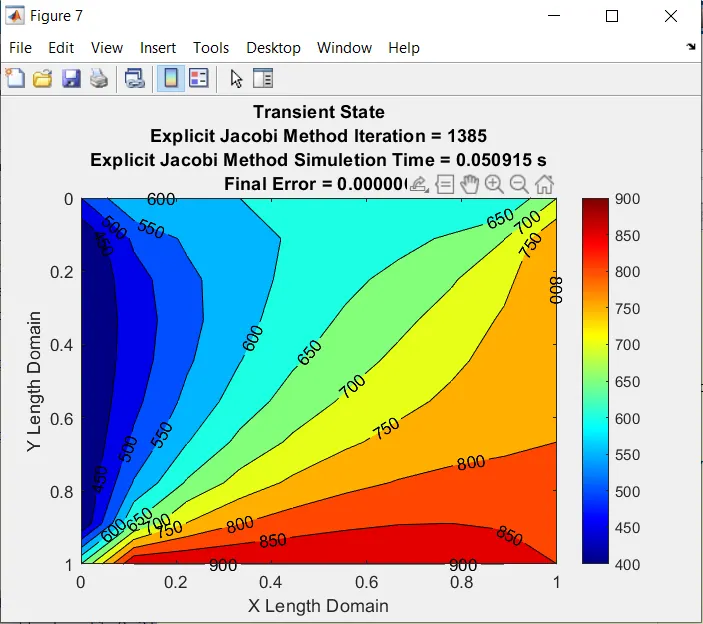

Explicit Jacobi Solver

-------------------------------------------------------------------------------------------------------------------------------------------

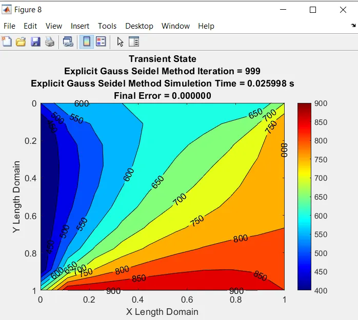
Explicit Gauss Seidel

-------------------------------------------------------------------------------------------------------------------------------------------

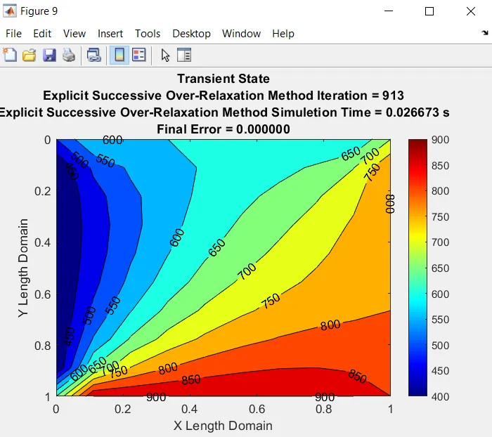
Explicit SOR

=============================================================================

% Main Code
%% Initiation
clear all
close all
clc

% Solving steady State 2D Heat Conduction 

%% Boundary Conditions

% Assumptions
nx = 10;
ny = 10;
% Square boundry of unit Length
L = 1; 
% Grid for x and y
x = linspace(0,L,nx);
y = linspace(0,L,ny);
[X, Y] = meshgrid(x, y);
dx = L/(nx-1);
dy = L/(ny-1);

% Absolute error criteria > tolerance
error = 9e9;
tolerance = 1e-4;

% Boundary conditions
T_L = 400;
T_T = 600;
T_R = 800;
T_B = 900;

% Intermediate points

T = 300*ones(nx,ny);

% Assigning boundary condition to grid

T(2:ny - 1, 1) = T_L;
T(2:ny - 1, nx) = T_R;
T(1, 2:nx - 1) = T_T;
T(ny, 2:nx - 1) = T_B;

% Calculeting Corner Values
T(1,1) = (T_T + T_L)/2;
T(nx,ny) = (T_R + T_B)/2;
T(1,ny) = (T_T + T_R)/2;
T(nx,1) = (T_L + T_B)/2;

% Preserving the value of orignal array
T_initial = T;
T_old = T;

%% Calculation 

alpha = 0.3;
t = 5;
dt = 1e-2;
% Assumption for steady state condition
k = 2*((1/dx^2) + (1/dy^2));
k1 = alpha*(dt/dx^2);
k2 = alpha*(dt/dy^2);

% Steady State analysis
 
for iter_method = [1 2 3]
    % Jacobi
    if iter_method == 1
        time = jacobi_steady(nx, ny, x, y, dx, dy,T_old, T, tolerance, error, k);
        % Gauss seidel
    else if iter_method == 2
        time = gauss_seidel_steady(nx, ny, x, y, dx, dy,T_old, T, tolerance, error, k);
        % Successive Over-Relaxation 
    else if iter_method == 3
        time = sor_steady(nx, ny, x, y, dx, dy,T_old, T, tolerance, error, k);
    end
    end
    end
end

% Unsteady or Transient State Analysis
% implicit form
for iter_method = [1 2 3]
    % Jacobi method
    if iter_method == 1
        time = implicit_jacobi(nx, ny, x, y, T_old, T, t, dt, tolerance, error, k1, k2);
        % Gauss seidel
    else if iter_method == 2
            time = implicit_gauss_seidel(nx, ny, x, y, T_old, T, t, dt, tolerance, error, k1, k2);
            % Successive Over-Relaxation
    else if iter_method == 3
            time = implicit_sor(nx, ny, x, y, T_old, T, t, dt, tolerance, error, k1, k2);
    end
    end
    end
end

% Explicit form
for iter_method = [1 2 3]
     % Jacobi method
    if iter_method == 1
        time = explicit_jacobi(nx, ny, x, y, T_old, T, t, dt, tolerance, error, k1, k2);
        % Gauss seidel
    else if iter_method == 2
            time = explicit_gauss_seidel(nx, ny, x, y, T_old, T, t, dt, tolerance, error, k1, k2);
            % Successive Over-Relaxation
    else if iter_method == 3
            time = explicit_sor(nx, ny, x, y, T_old, T, t, dt, tolerance, error, k1, k2);
    end
    end
    end
end

Result

Steady-State Methods

From the output graphs computed we can say that the Successive over-relaxation method is the most efficient as it has the lowest simulation time and several iterations when compared to the Jacobi and gauss seidel methods. And also note that the final error for the SOR method is the lowest compared to the other two methods for the steady-state solver. As it is a variant of Gauss seidel and Jacobi methods and uses the results from them to further improve the result and it uses a relaxation factor to do so. Depending on the factor, the number of iterations, and the accuracy of the result determined, this factor is experimentally determined.

Transient State Methods

Implicit Condition

Under this condition we notice the same trend of the results, the SOR method is the most accurate and Efficient to solve and compute in terms of the simulation time and the iteration computed by the solver.

Explicit Condition

Yet again a similar trend repeats itself as an observer in the above 2 cases but the simulation time and the error are considerably low (denomination not computed in the results).

Thus we can conclude that the Transient Explicit State with successive over-relaxation methods is the superior method for 2D heat exchange through conduction.

Report Link: https://docs.google.com/document/d/1ZoqkIi9mPS6vhk6vOBPVHaqEdD3QhiD_ZzwacPxUn0k/edit?usp=sharing