Introduction to GUI based CFD analysis using ANSYS FLUENT

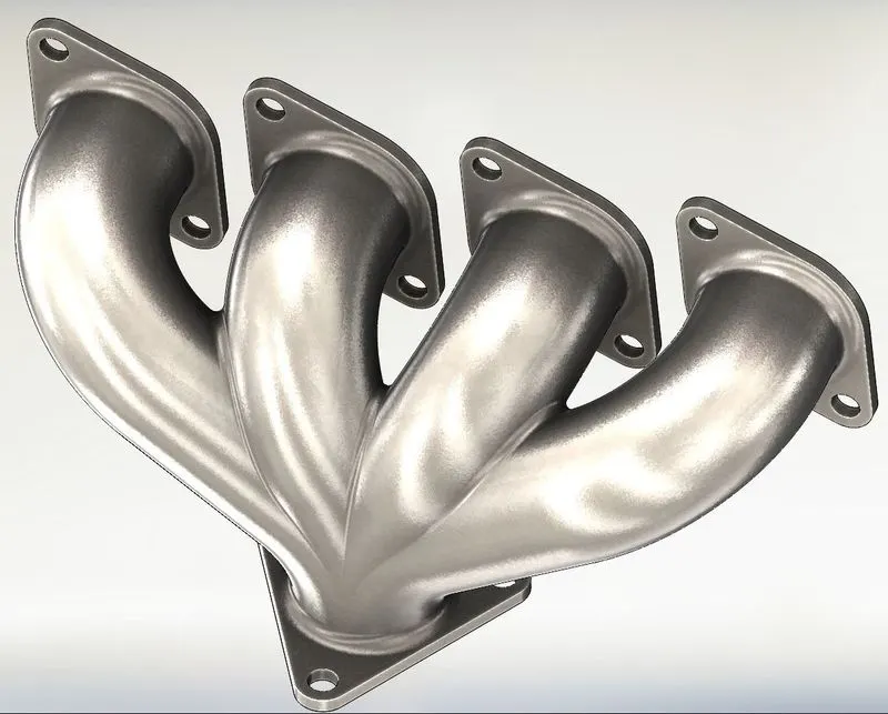
Exhaust Port

CHT Analysis on Exhaust Port

Introduction

Conjugate Heat Transfer

Heat transfer in solids and heat transfer in fluids are combined in the majority of the applications. This is because the fluid flows around solids or between solid walls and because solids are immersed in a fluid.

The term conjugate heat transfer is used to describe a process that involves a variation of temperature between solids and fluids, due to thermal interactions between the solids and fluids. The exchange of thermal energy between 2 physical bodies is called the study of heat transfer, the rate of transferred heat is directly proportional to the temperature difference between the bodies. A typical example is the heating or cooling of the solid object by the flow of air in which it is immersed or some other example includes conduction through solids, free and forced convection in the fluids and thermal radiation.

CHT corresponds to the combination of the heat transfer in solids and heat transfer in fluids. In solids often conduction dominates and in fluids convection dominates. Efficiently combining the heat transfer in the fluid and solids is key to designing effective coolers, heaters, heat exchangers, etc. forced convection is the most common way to achieve a high heat transfer rate. In some applications, the performance is further improved by combining convection with phase change.

The accurate modes, material properties, flow regimes and geometrical configurations enable the analysis of temperature fields and heat transfer. Such a description is also the starting point for the numerical simulation that can be used to predict conjugate heat transfer effects or to test different configurations in order, for example, to improve the thermal performance of a given application.

Application of CHT

The internal combustion engine industry; is moving towards simulating the entire system rather than independent components. The accuracy of the predicted combustion in the cylinder is dependent on the temperature boundary conditions in the cylinder.

Electromobility

Effective cooling strategies are critical for various components of an e-mobility system. Electric motors have high power density and thus generate a significant amount of heat. If a motor is not properly cooled, high temperature in the motor can cause the demagnetization of the permanent magnets and the breakdown of the winding insulation.

Aftertreatment

Predicting and mitigating urea deposit formation is a key challenge in Urea/SCR after-treatment systems. When the urea-water solution is sprayed into the engine exhaust system, it impinges on the wall as a liquid film. The decomposition of Urea and the formation of undesirable deposits are highly dependent on the wall temperature, and the transfer between the film and the wall is important to capture. Protecting the wall temperature helps you identify areas that are vulnerable to wall deposition.

Pumps and compressors

Resolving the spatially varying surface temperature distribution in the pumps and compressors improves the accuracy of the simulation and provides useful temperature data. For example, in a twin-screw compressor, thermal expansion affects the clearance between the rotors. If the effect is not captured the simulation will incorrectly predict leakage flows and lower the accuracy of your results.

Problem

Give a brief description of why and where CHT is used.

Maintain the Y+ value according to the turbulence model and justify the results.

Calculate the wall/surface heat transfer coefficient on the internal solid surface and show the velocity and the temperature contour in the appropriate areas.

How are the HTC predictions from the simulation verified to be correct? On what factors does the accuracy of the prediction depend?

Solution

Geometry

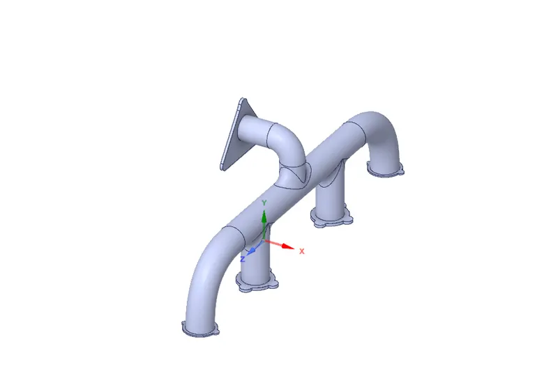
The geometric setup of the model is such that the extracted volume, that is the fluid and the solid part, share information to simulate the energy transfer.

That is done by keeping the volume (solid and fluid) in a separate component, and ensuring the mesh quality and continuity with the ‘share topology’ and ‘share prep options’.

As mentioned this will allow the 2 geometric volumes to share the information amongst each other effectively and increase the accuracy of the heat transfer results through the solid.

Meshing

Meshing is done in 2 ways, first, a baseline mesh is generated and then the simulation is performed and then the mesh is refined and then the simulations are run again.

Baseline Mesh

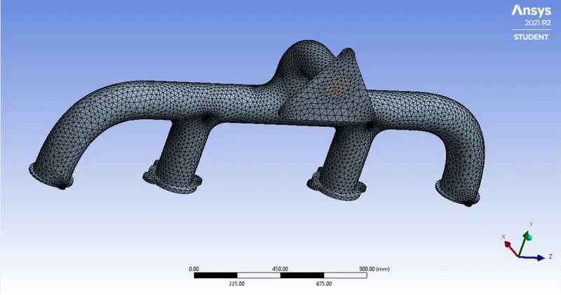
The named selection is used to name the boundary condition, the baseline mesh allows us to get a benchmark for the problem before refining the mesh and generating the rough results.

The baseline mesh does not include any inflation layer or body sizing modification, a sample mesh is generated and simulation is done. The total number of elements is 136735.

Refined Mesh

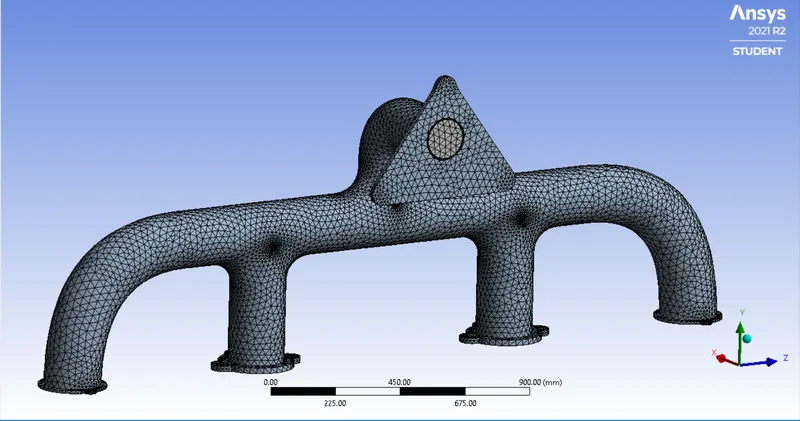
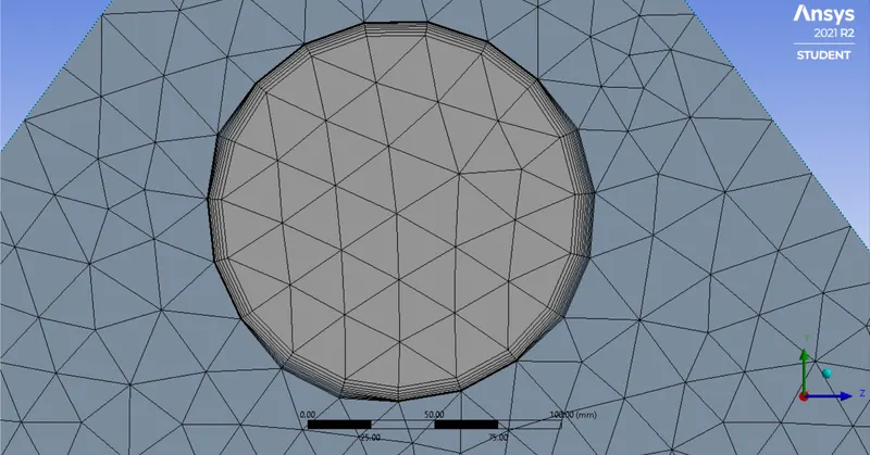
One more named selection is added which is at the interface of the solid volume and fluid volume. An Inflation layer of 5 layers is added on the interface of the solid volume and the fluid volume, which allows accurate results for fluid properties at the boundary. Body sizing is done on the internal volume or the fluid volume. This takes the number of elements to 252180 and provides accurate results for the simulation.

Setup

Baseline setup

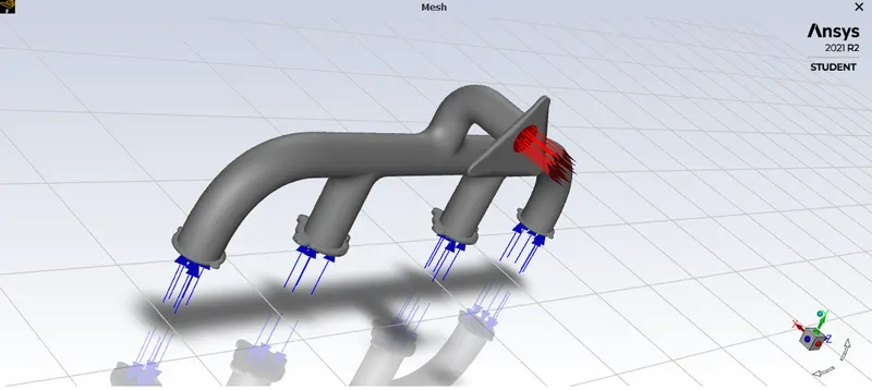
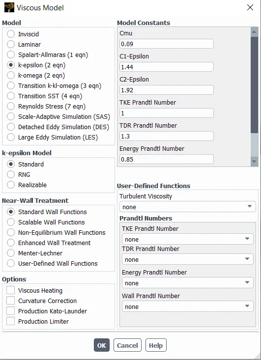
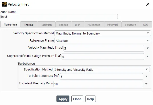
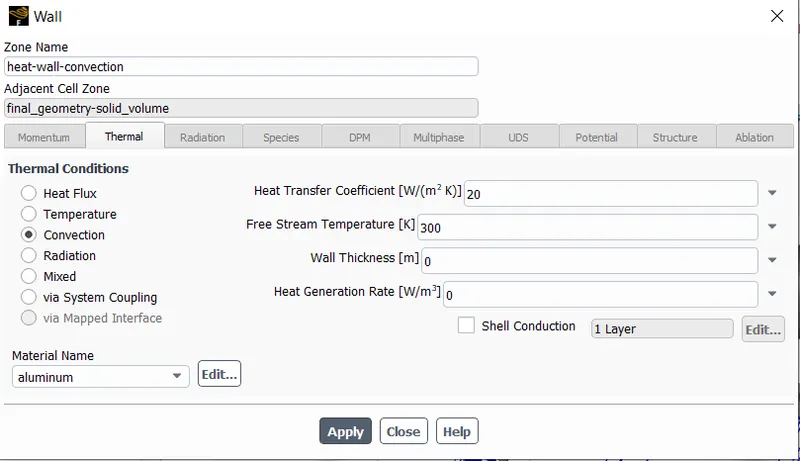
In the baseline simulation, the plots and contours are generated, the K-ε viscosity model is used, along with this the pressure-based model is used and then we initialise the model hybrid. We simulate for 250 iterations and get the results.

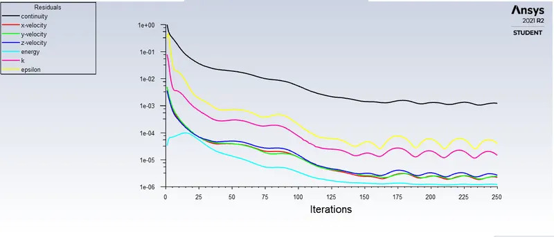
Scaled Residuals

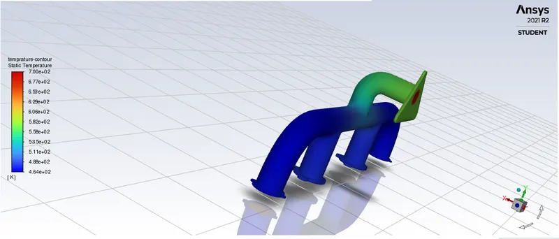
Temperature contour

Refined setup

In the refined simulation, the plots and contours are generated, the K-ε viscosity model is used, along with this the pressure-based model is used and then we initialise the model hybrid. We simulate for 250 iterations and get the results.

The refined mesh will allow the simulation to generate more accurate results and better visualisation of the results at the boundary of the solid and the volume of the fluid.

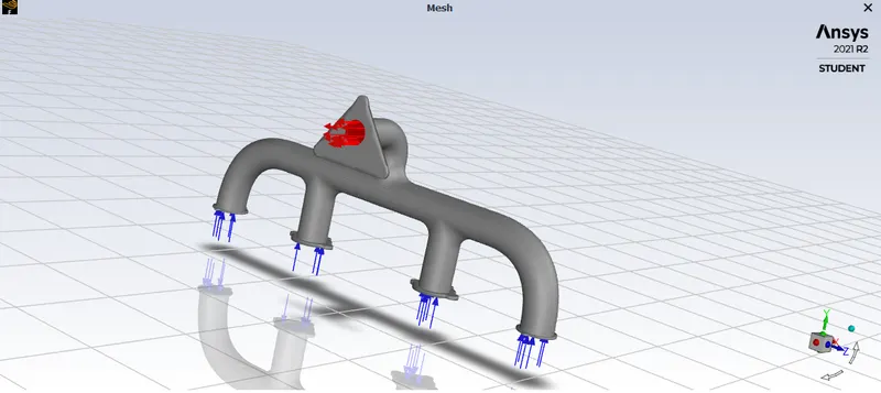
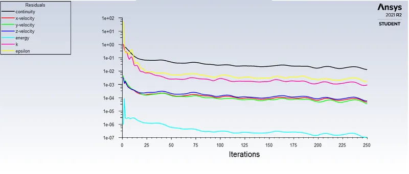
Scaled Residuals

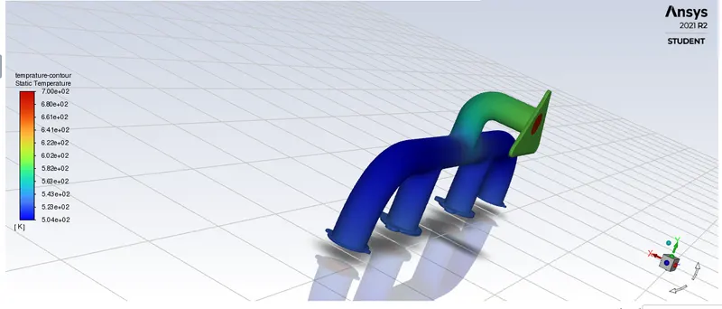
Temperature contour

Result

Baseline results

This gives us a rough estimate of the results and this is a benchmark to check when the results are calculated when the mesh is refined. The results we receive are the temperature contour, velocity field line field and temperature and velocity contour along the plane in the outlet, we also plot the temperature heat transfer coefficient along the wall.

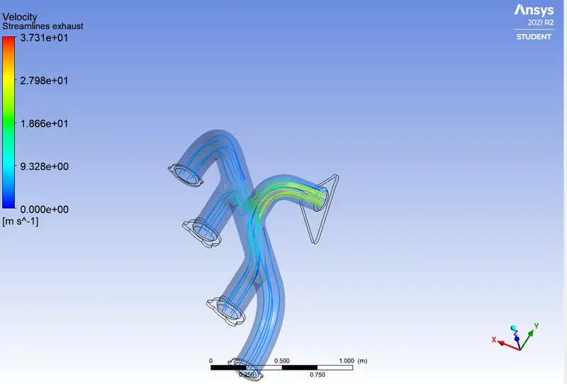
Baseline velocity field.

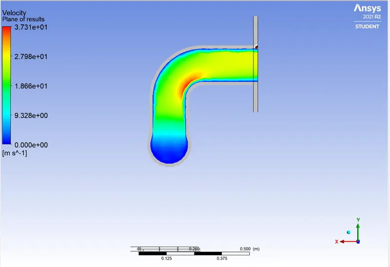
Baseline velocity distribution along the outlet pipe.

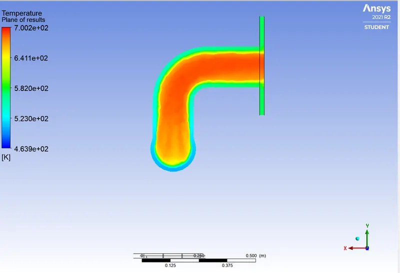
Baseline temperature distribution along the outlet pipe.

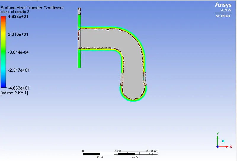
The surface heat transfer coefficient for the baseline case is distributed along the wall.

Refined results

With the refined results, we can get an exact result for the heat flow, temperature distribution, velocity distribution, and heat transfer coefficient.

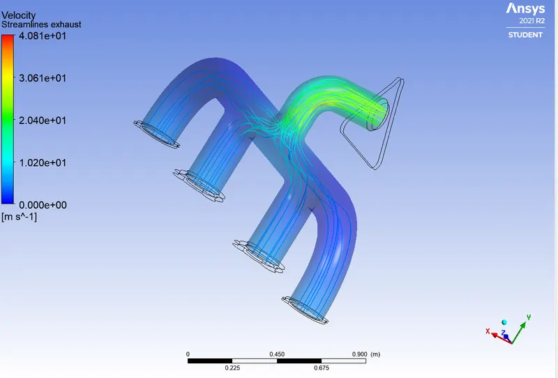
Baseline velocity field

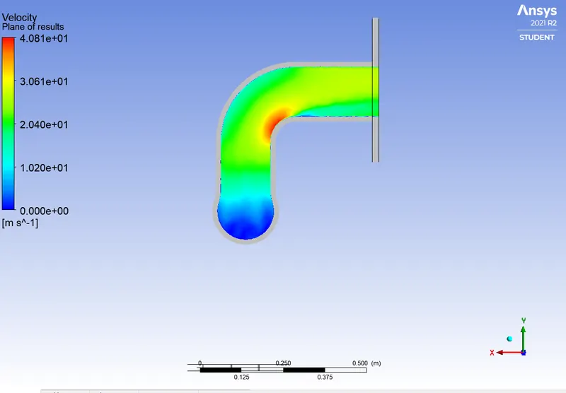
Baseline velocity distribution along the outlet pipe.

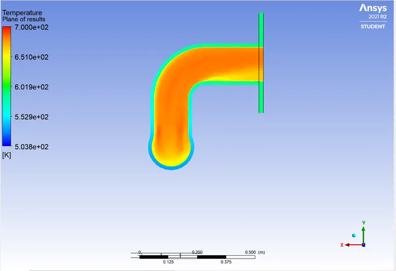
Baseline temperature distribution along the outlet pipe.

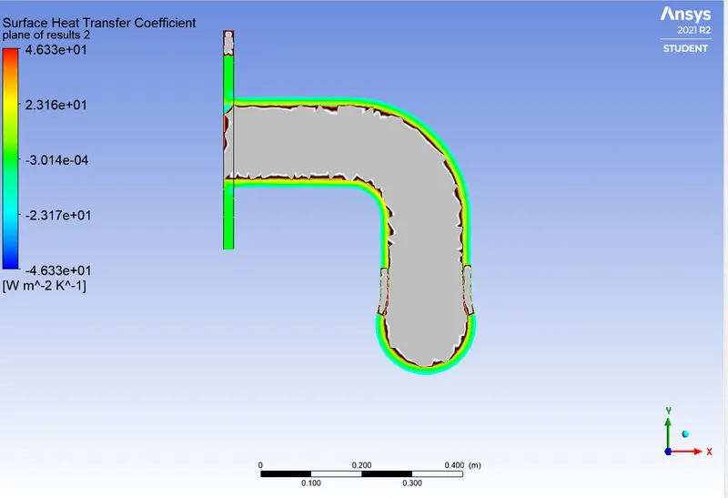
The surface heat transfer coefficient for the baseline case is distributed along the wall.

Verification of HTC Prediction

The Re. is produced in the range of 10^3 to 5*10^4 in typical flow conditions on vehicle exhaust systems. Especially in the exhaust manifold runners, the exhaust flow frequently approaches the Re 2300 zone. Despite this, the flow remains turbulent since it has passed through a significant obstruction. The exhaust valve, as well as the flow pulsation effects that endure, do not favour the transition to the laminar area.

According to the Sieder Tate relation which correlates the Nu number with the Re and Pr,

Nu = 0.027 (Re^0.8) Pr^(1/3)

The Nusselt number is a function of both the Renolds and Prandtl numbers.
Because the turbulent boundary layer at the curve at the output port is shallow, the flow reaches its maximum velocity at the bend, resulting in a larger Renolds number.
Now Nu = h*L/K
The value of h will grow while the pipe length and heat conductivity remain constant, and the Nu will increase as Re increases.
According to our findings, the higher the velocity, the higher the heat transfer coefficient, and hence we believe our findings are valid.

The factors affecting the quality of the Predictions:

• More refined mesh leads to better results.
• Use inflation layers and apply proper Boundary conditions.
• Proper selection of turbulence model according to y+ values.

Conclusion :

1. Correct choosing the value y+ which satisfies the turbulent model, by effectively capturing the velocity and temperature at the boundary wall interface.
2. Meshing at the junction of the solid and fluid domain. With a definite value of y+, the no inflation layers and the growth rate determines the smooth flow of heat transfer between the zones.
3. By the above temperature contour it shows that the maximum temperature on the outer wall is at the outlet region of the model because we have 4 inlet and only one outlet velocity at the outlet is increased. Temperature is proportional to the average kinetic energy of the molecules of the gas. So when temperature increases fluid velocity increases and vice-versa.
4. While comparing temperature control between the base mash and the refined mash we observe that the temperature will be uniformly distributed in refined.
5. Velocity is greater in the refined match compared to base mesh because in refined mesh we provide an inflation layer so it can capture more accurate velocity at the sharp edge.
6. The wall heat transfer coefficient is also greater in refined mash compared to base mesh because again we provide an inflation layer in the refined mash, so it can capture a more accurate heat transfer coefficient near the wall.
7. So we can say that if we create mesh properly around the model then we definitely got much more accurate results.

Report link: https://docs.google.com/document/d/1RVgseQTzGk-44yBv3ez9s_hKrn-hhpgg4Q1L1Kt7G5Q/edit?usp=sharing