Week 5 - Rayleigh Taylor Instability
Introduction to GUI based CFD using ANSYS FLUENT
Rayleigh Taylor Instability
Mixing of Two fluids in a Control Volume
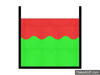
RT instability is the instability of an interface between two fluids of different densities which occurs when the lighter fluid is pushing the heavier fluid, example includes the behaviour of water suspended above oil in the gravity of Earth, mushroom clouds like those from a volcanic eruption and atmospheric nuclear explosion, Supernova explosion in which expanding core gas is accelerated into denser shell gas, instabilities in plasma fusion reactors and internal confinement fusion.
Mixing of water and oil is a common example that we can observe for the RT instability, it may be modelled by 2 completely plane-parallel layers of immiscible fluid, the denser the top and least dense the bottom is when subjected to gravity. The stability of this equilibrium is sensitive to any disturbance or change in the interface. If supposedly a small volume of the heavier fluid is displaced downwards, an equal volume of the lighter fluid will displace upwards, with this, a drop in the potential energy is observed compared to the initial condition, this will cause a chain reaction of the fluids mixing an trying to achieve a state of lower potential energy which is lower than their initial state as more fluid will exchange, the lighter fluid will form bubbles and replace the volume in the heavier fluid moving upwards, and under the effect of gravity the denser mass will sink downwards. These results are also used when we want to accelerate a less dense fluid in a more dense fluid, example is expanding bubbles underwater and underwater explosions.
Saffman-Taylor Instability
This instability is the formation of patterns in a morphologically unstable interface between 2 fluids in a porous medium. This situation is most often encountered during the drainage process through a medium such as soil. It occurs when a less viscous fluid is infected, displacing the more viscous fluid, in the inverse situation, with the more viscous displacing the other, the interface is stable and no instability is seen. Essentially the same effect is seen under gravity if the interface is horizontal and separates 2 fluids of different densities, the heavier one being the above the other, the system evolves until a single finger forms whilst in the radial configuration, the pattern grows to form fingers by successive tip-splitting.
Richtmyer-Meshkov Instability
Observed when 2 fluids of different densities are accelerated impulsively. Normally this is by the passage of shockwaves. The development of the instability begins with a small amplitude disturbance which has linear growth with time initially. This is followed by a nonlinear phase with bubbles appearing in the case of light fluid penetrating the heavy fluid, and with spikes appearing in the case of the heavy fluid penetrating the light fluid. A chaotic phase is eventually reached and the 2 fluids mix. This can be considered the impulsive-acceleration limit of Rayleigh-Taylor Instability.
Kelvin-Helmholtz Instability
It occurs when there is velocity shear in a single continuous fluid, or additionally where there is a velocity difference across the interface between 2 fluids. A common example is seen when the wind blows across a water surface. The velocity constant manifests as waves. The other examples are cloud formation on Earth, the Red spot on Jupiter, etc.
Mushroom Cloud
The mushroom cloud is a distinctive mushroom-shaped cloud of debris, smoke and usually condensed water vapour resulting from a large explosion. The effect is most commonly associated with a nuclear explosion but any sufficiently energetic detonation or deflagration will produce the same effect. They can be caused by powerful conventional weapons, like thermobaric weapons, Volcanic eruptions and the meteorite impact can produce them naturally.
Mushroom clouds result from the sudden formation of large volume low-density gases at any altitude, causing an RTI. The buoyant mass of gas rises rapidly, resulting in turbulent vortices curling downwards about its edges, forming a temporary vortex ring that draws up a central column, possibly with smoke, debris, and/or condensed water vapour to form a ‘mushroom stem’. This mass eventually reaches an altitude where it is no longer of lower density than the surrounding air, at this point, it disperses, drifting back down. The stabilization altitude depends entirely on the profile of the temperature, dew point and wind shear in the air at and above the starting altitude.
The Plateau–Rayleigh instability
Often just called the Rayleigh instability, explains why and how a falling stream of fluid breaks up into smaller packets with the same volume but less surface area. It is related to the Rayleigh–Taylor instability and is part of a greater branch of fluid dynamics concerned with fluid thread breakup. This fluid instability is exploited in the design of a particular type of inkjet technology whereby a jet of liquid is perturbed into a steady stream of droplets.
Practical CFD models
- The smoothed particle hydrodynamics method is a computational method used for simulating the mechanics of continuum media, such as solid mechanics and fluid flows. SPH is gaining popularity to model fluid motion as well. Due to its benefits over the traditional grid-based techniques. It conserves the mass without any additional computation as the particles involved themselves represent mass. It also computes pressure from weighted contributions of neighbouring particles rather than by solving linear systems of equations. Lastly, unlike grid-based techniques, which must track fluid boundaries, it creates a free surface for two-phase interacting fluids directly since the particles represent the denser fluid and space represents the lighter fluid.
- Single-fluid model, A typical approach used for the analysis of two-phase flows is a mixture model, i.e. the individual flow phases are resumed to behave as a flowing mixture described in terms of the mixture properties. The applied single-fluid model is a 5-equation model consisting of the mass, momentum and energy equation for a vapour/liquid mixture, and two equations describing the formation and growth of the liquid phase.
- Two-fluid models, separate sets of governing equations for vapour and liquid phase have been used. The interaction between the droplets and heat exchange between the liquid phases and the solid boundary is not modelled here as well. Additionally, the velocities played between the vapour and the liquid phase is in this model taken into account.
- Turbulence models are needed to predict the average mixing behaviour and flow that is on average one or two dimensional. The approach to the construction of the tile turbulence model is guided by experimental behaviour. The equations governing turbulent flow can only be solved directly for simple cases of flow. Foremost real-life turbulent flow, CFD simulation uses turbulent models to predict the evolution of turbulence. These turbulence models are simplified constitutive equations that protect the statistical evolution of the turbulent flow.
Problem
- What are some practical CFD models that have been based on the mathematical analysis of Rayleigh Taylor waves? In your own words, explain how these mathematical models have been adapted for CFD calculations.
- Perform the Rayleigh Taylor instability simulation for 2 different mesh sizes with the base mesh being 0.5 mm. Compare the results by showing the animations( Attach them from your google drive). Observe the differences in the animation and explain the effect of mesh size on simulation. Also, explain why a steady-state approach might not be suitable for these types of simulation.[ Choose Air and Water for this simulation]
- Run one more simulation with water and user-defined material(density = 400 kg/m3, viscosity = 0.001 kg/m-s) for refined mesh.
- Define the Atwood Number. Find out the Atwood number for both the cases and explain how the variation in Atwood number in the above two cases affects the behaviour of the instability.
Solution
Geometry
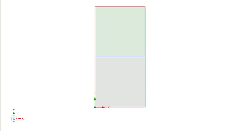
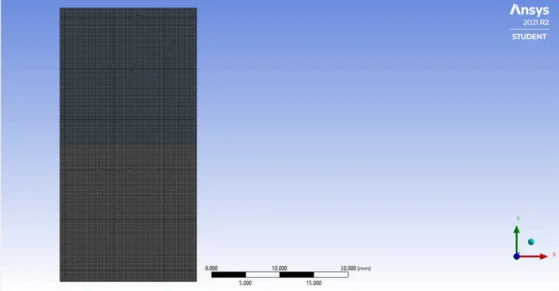
We generate the geometry in the Spaceclaim and the model is a 2-D figure which is 20X40 mm and the 2 phases of the geometry are separated with each having a patch of 20X20 mm the upper domain is for water and the lower domain is for air.
With the help of the share topology command/tool, we allow the share of data between the 2 domains.
Meshing
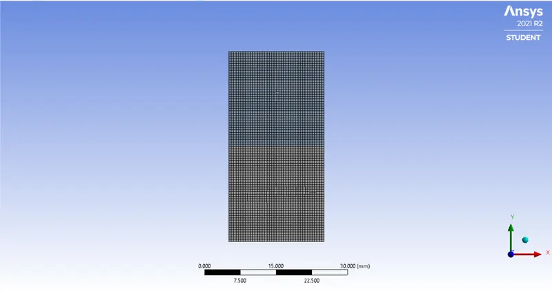
The meshing is done for 3 element sizes to get 3 different refinement levels one will be the baseline mesh with the element size of 0.5 mm and the other 2 will be further refined from this within the licence limit.
Baseline Mesh
The baseline Mesh will provide a benchmark for the other cases to compare the results to, the number of nodes is 3321 and the number of elements is 3200.
First Refined Mesh
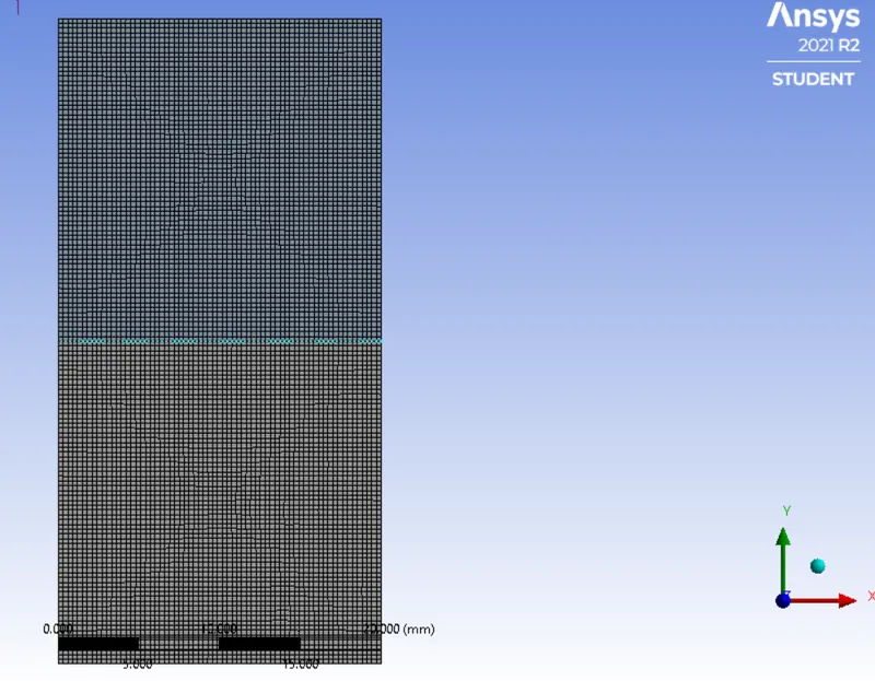
We will reduce the element size to 0.3 mm and keep all the other conditions the same. The number of nodes is 9180 and the number of elements is 8978.
Second Refined Mesh
We will reduce the element size to 0.2 mm and keep all the other conditions the same. The number of nodes is 20301 and the number of elements is 20000.
Setup
Baseline Setup
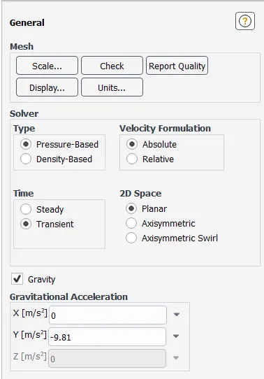
We use a pressure-based solver and transient condition in the presence of gravity.
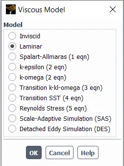
The viscosity/turbulence model used is the laminar model since the velocities are very slow.
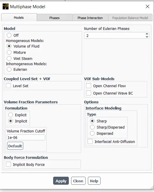
We also implement the multiphase model, Volume of the fluid model with the implicit formulation is used, we also rename the phases of the mixing fluids like air and water.
Now the model is initialised and we use standard initialisation, after which we distribute the patch conditions of alpha, 0 for air and 1 for water.
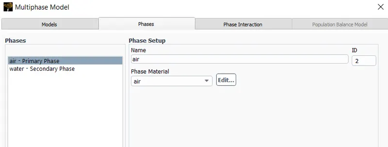
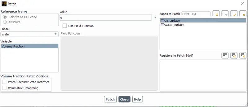
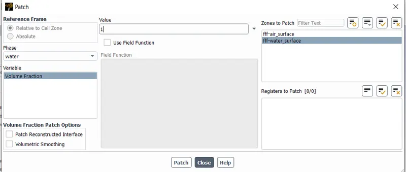
Timestep size is 0.005s and the number of timesteps is 1000
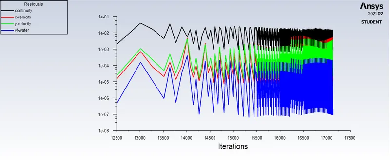
Baseline Residuals
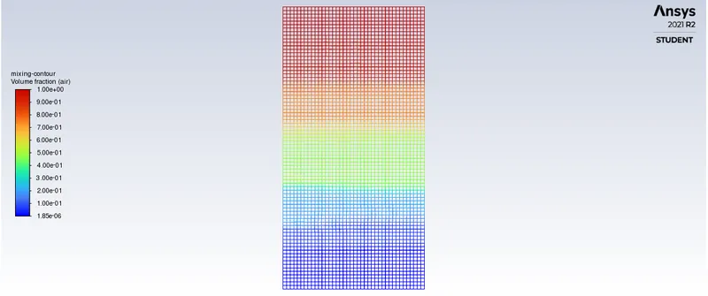
Baseline phase contour
First Refined Setup
For the setup, the conditions and the models remain the same and we patch the regions in the same way after the initialisation,
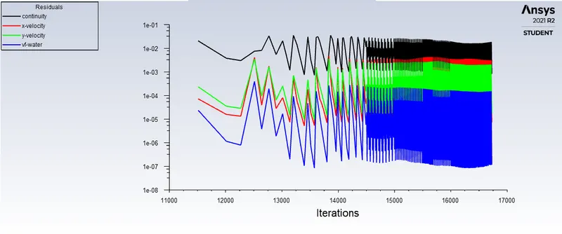
First Refined Residuals
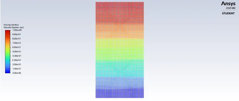
First Refined Contour
Second Refined Setup
For the setup, the conditions and the models remain the same and we patch the regions in the same way after the initialisation,
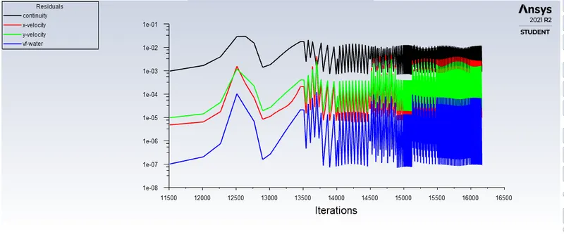
Second Refined Residuals
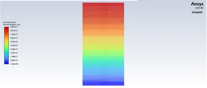
Second Refined Contour
User-Defined Case
The meshing will be the Second Refined meshing condition and the setup will remain unchanged the conditions for the user-defined case will remain the same as the Second refined setup, only the material properties will change for the fluid that replaced air.
Properties of the User Defined fluid are as follows,
Density = 400 Kg/m^3
Viscosity = 0.001Kg/m-s
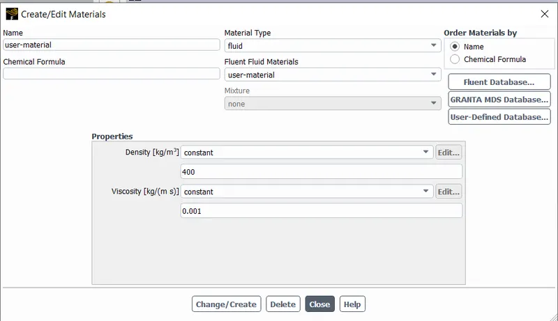
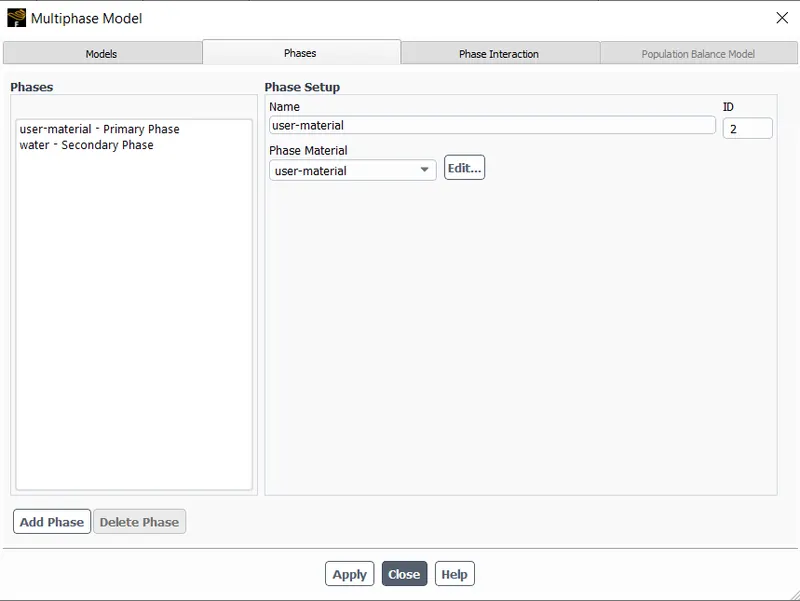
The setup is initialized and patched and we run it for 1000 iterations with a time step of 0.005s
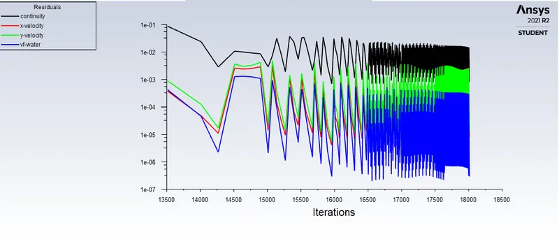
User-Defined Residuals
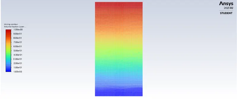
User-Defined Contour
Conclusion
In the above cases, the simulation starts with a state of hydrostatic equilibrium and the RT Instability is observed at the interference when the lower density fluid pushes a higher density fluid due to which formation of shock wave at the interface takes place. Formation of air bubbles starts taking place, which compresses the heavy fluid around it, due to which shock waves of multidimensional fashion generate and it gets more strong as it moves upwards.
The increase in the quality of the mesh increases the quality of the results and makes it more accurate, the replacement of fluid that takes place leads to the generation of bubbles and vortices which rises with time in the volume. The trapped air bubbles, the vortices and waves are much more refined in Case 3 (Second refinement) when they are trapped in the lower region during the initial stages and generate shock waves as they go up. In the end, the 2 phases are separated with some diffusion left behind.
Incompatibility of Steady-state approach
The difference between the steady and transient is that you can't see the small-time variation of instability. The steady-state simulation is performed if we are concerned more about the final state results or the equilibrium state. In RT-Instability CFD models, we are more concerned to learn about the transition of the irregularities that starts developing when we pour high dense fluid upon low dense fluid under gravity effect so, by using transient solver along with refined mesh of the model, we can compute the smooth transition of irregularities that takes place at the interface of the fluids. The final state results for both the steady-state and transient state will be the same.
In this problem we are observing the instabilities when it is occurring so we are not concerned about the final answer because the steady-state is more into capturing the final results but by transient, we can see the behaviour of the solution and every instant such that capturing bubbles, Vortex and shockwaves. So this is the reason why transient is more suitable than the steady-state model
Atwood Number (A)
A dimensionless number in fluid dynamics is used in the study of hydrodynamics instability in density satisfied flows. It is a dimensionless ratio defined as,
A = ⍴1 - ⍴2 / ⍴1 + ⍴2
Where ⍴1 = density of the heavier fluid and ⍴2 = density of the lighter fluid
A = 1000 - 1.25 / 1000 + 1.25 = 0.9975
It is an important factor for the study is of RT instability. For Atwood numbers close to 0, RT instability takes the form of an asymmetric ‘finger’ of fluid; for the Atwood number close to 1, the much lighter fluid ‘below’ the heavier fluid takes the form of a large bubble-like structure.
The Atwood number we calculated is close to 1 and from the simulation results, it is found that when a high-density fluid (water) is poured upon a low-density fluid (air) under gravity, the formation of air bubble-like structures take place which travels towards the upward region in the form of waves and some get trapped at the lower regions during the initial stages, which afterwards try to move to the upper region and at the end, both phases get separated with some diffusion left in the middle region between them and this result is validated by the Atwood number calculated,
Case 1
Heavier fluid (water)
Density 1 = 998.2 Kg/m^3
Lighter fluid (air)
Density 2 = 1.225 Kg/m^3
Atwood no. (A) = (Density 1 - Density 2)/(Density 1 + Density 2) = 0.996
Case 2
Heavier fluid (water)
Density 1 = 998.2 Kg/m^3
Lighter fluid (Used defined material)
Density 2 = 400 Kg/m^3
Atwood no. (A) = (Density 1 - Density 2)/(Density 1 + Density 2) = 0.427
The Atwood number is an important parameter in the body of RT instability and Richtmyer-Meshkov instability. In RT instability, the penetration distance of heavy fluid bubbles into the light fluid is a function of acceleration time scale. A*g*t^2, where ‘g’ is acceleration due to gravity and ‘t’ is time.
Effect of ‘A’ on the instability of the uniform interface
The evaluation of a uniform interface subjected to a perturbed shock wave has been experimentally studied over a range of Atwood numbers 0.22 <= A <= 0.68 and Mach numbers 1.2 <= M <= 1.8 using a vertical shock tube. The perturbed shock wave is produced by diffracting a planar incident shock over a rigid cylinder. The wave patterns of the perturbed shock are captured by high-speed shadowgraphy while the evaluation of the shock interface is captured by planar Mie scattering. Besides the formation of a cavity and two steps, an apparent counter-rotating vortex pair emerges on the shock interface due to the baroclinic vorticity deposition, as both the Atwood number and Mach number increase, Quantitatively it is interesting to note that the amplitude growth rate of the shocked interface decreases with increasing the Atwood number, which is fundamentally different from the results related to the classical RM instability. This notable feature is explained by the approximation of an oblique shock hitting a uniform interface. For weak shock, a suitable time scaling is employed to collapse experimental data irrespective of the Atwood number difference.
Video link: https://youtu.be/WqAW_qLVy-c
Report link: https://docs.google.com/document/d/1qqWHJ0y34-uRm76PN0-4_qcMOCxRYNGzydm8Z1k6yk0/edit?usp=sharing