Finite Volume Method

Literature review for Finite Volume Method

Introduction

• The Finite Volume Method is applied on a control volume such that the governing equation is valid over the entire volume. It is used to represent and evaluate PDEs in the form of algebraic equations.

1. The value of variables is represented at the centre of the volume.
2. Allows the use of non-uniform mesh or unstructured mesh. No assumptions are made over the shape of the volume.
3. The volume integral in the PDE that contains divergence terms is converted to the surface integral by using the divergence theorem.
4. These terms are then evaluated as the flux at the surface of each finite volume. The flux entering a given volume is identical to the flux leaving the adjacent volume.
5. The conservative properties are pre-embedded in the solution scheme itself, whether it is applied on a small arbitrary volume in the system or the system itself.
6. All the physical properties/flow field variables are conserved whether it is momentum, mass or energy in the flow.
7. It gives us the liberty that instead of writing the governing equation for every point we do the computation for the control volume.
8. The initial process involves the division of the given volume into the small control volumes.

The solution is generated using the following steps;

1. Achieve the integral form of the governing equation.
2. Apply the gauss divergence theorem.
3. The achieved discretized form can be solved via flux terms.

Consider a steady state heat equation with heat generation;

∂ / ∂x [ (∂T / ∂x)] + S = 0 -(1)

Where S = source term; = thermal diffusivity term; ∂T / ∂x = is the temperature gradient along the x-axis.

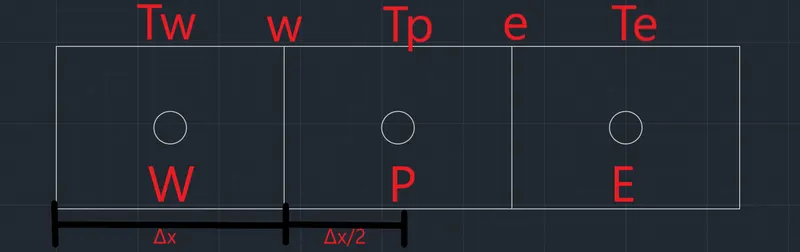
Equation (1) is valid at every point in the domain, i.e. it is valid in the entire control volume.

Consider a small volume ‘dv’ multiplied with the governing equation and integrated it for the entire control volume.

If the equation stands true for the assumed volume ‘dv’ then it will stay true for the entire control volume.

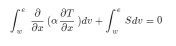
We assume dv = A.dx

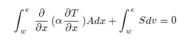-(2)

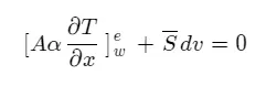-(3)

S(bar) is the average value of the source term.

-(4)

Let ‘alpha’ be a constant

-(5)

Which can also be interpreted as [heat flux out] - [heat flux in] + source term = 0

Solver Scheme

There are some schemes used to solve the Finite Volume Problem.

Gradient Scheme

When we calculate the temperature gradient in the east face we use temperature from the neighbouring points trying to evaluate or numerically represent the gradient of temperature is called the gradient scheme.

Extrapolation Scheme

Similar to the gradient scheme this uses values of flow field variables/ unknown from one side in determining the point of concern for approximation.

First Order Upwind Scheme (FOU)

Constant linear extrapolation, where only one upstream neighbour is used. This gives a result that is a straight line that has a ‘0’ slope, because of which the value at e = value at p.

Second Order Upwind Scheme (SOU)

Computed using 2 upstream neighbours. And is comparatively accurate.

Interpolation Scheme

Process of estimating the values at unknown points by using the points with known values and sample points on either side of the unknown point.

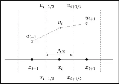
In FVM interpolation schemes are used to find values of the volume and the surface integral requires to find the value of the unknown variable at the points other than the nodes.

Upwind Interpolation Scheme

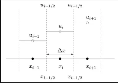
It takes into account the direction of fluid flow and based on it, the value of the solution variable at the face is approximated by its value at the upstream computational node.

This scheme is for approximating the value of a variable (say ‘f’) at each face of the control volume given by,

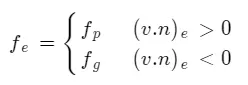
Generally used in convection domain problems,

v>0

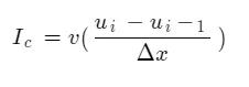
This is a Backward difference

v<0

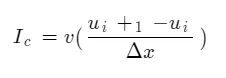Forward difference

In a first-order flux approximation, the leading truncation error resembles a diffusive flux.

d( ∂u)/(∂x) where d = vΔx/2 being a numerical diffusion coefficient.

Linear Interpolation Scheme

To approximate the value at the Cv face centre by linear interpolation of the values at the 2 nearest computational nodes. This is similar to the central difference scheme on first order divergence, and hence it is also known as the central difference scheme. This leads to the simple approximation of the evaluation of the gradient required for the evaluation of diffusive fluxes.

Quadratic Upwind Interpolation Scheme

This approximates the value at the Cv face centre by quadratic interpolation of the values, at 3 nearest computational nodes. It is third-order accurate for both uniform and nonuniform grids.

Hybrid Interpolation Scheme

Blend of CSD and USD, based on Peclet number.

Total Variation Diminishing Scheme

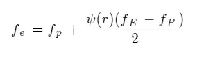
Here ψ is the flux limiter.

Flux Limiter

We study the behaviour of numerical schemes to capture shock and discontinuity that arises in hyperbolic equations.

For conservative fluid flow, it is observed that low order schemes are usually stable but quite dissipative around the points of discontinuity or shocks while the higher-order schemes are unstable and show oscillations in the vicinity of discontinuity or shocks.

Achieving higher order is not possible without oscillations. Flux limiters are used to fine-tune the higher order and lower order schemes in such a way that the resulting scheme gives a higher-order accuracy in the smooth region of the flow and maintains the first-order accuracy in the vicinity of shock and discontinuities

Report link: https://docs.google.com/document/d/1zPsDBUsEkVek7l9qoQC1cyKB8L2yYgs5NVIVODEUF9s/edit?usp=sharing