Mixing Tee

Use ANSYS FLUENT to Simulate the Mixing of Fluid in T-joint

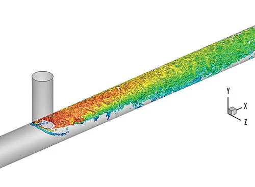
AIM

To simulate the flow of air through a mixing tee. We have 2 different conditions.

1. Effect of different ratios of momentum, velocity on the mixing (variation in inlet velocities).
2. The effect from extending the length of pipe, after the mixing (variation in the length of the pipe).

Introduction

In industrial process engineering, mixing is a unit operation that involves the manipulation of a heterogeneous physical system with the intent to make it more homogeneous. Mixing is performed to allow heat or mass transfer to occur between one or more streams, components, or phases. Modern industrial processing almost always involves some form of mixing. A mixing tee is a type of mixing mechanism.

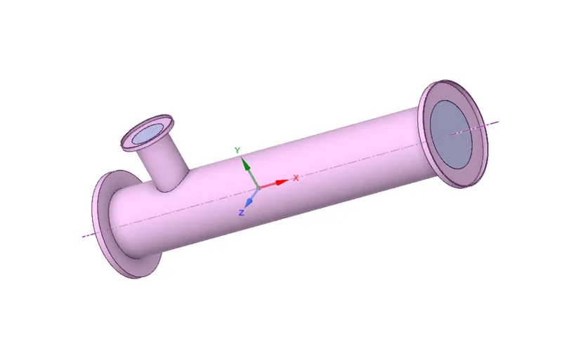
Mixing Tee’s are widely used in cases where 2 fluid streams with different physical and/or chemical properties mix. When there is a large temperature difference between the 2 streams, large metal temperature fluctuations can occur in the region where the 2 fluids mix.

The mixing Tees are widely used in petrochemical and HVAC industries, etc. The standard deviation of temperature fields is also computed. The effects of the mesh size, turbulence model on results were examined.

Problem

1. Create 2 versions of mixing tees, of varying lengths.
2. Steady-state simulation to compare the mixing efficiency when hot inlet temperature is 36°C and the cold inlet is at 19°C.

The momentum ratio is said to be the ratio of velocities of the air coming from either of the inlets.

Solution

We will be computing for three cases. The first case will be a ‘control’. In this control, we will assume the standard conditions, like small length with an inlet velocity of the cold air at 3 m/s. This is followed by a case where the momentum ratio is increased to 2 and 4. The third case has the inlet velocity of cold air as 3 m/s but the length of the pipe is increased after the air from both the inlets starts mixing. Same as earlier the momentum ratio is increased to 2 and 4 in this model as well.

Case setup

Short Tee, Momentum Ratio 2;

CAD Cleanup with SpaceClean, this app is used to clean the generated model and get the relevant volume from the model.

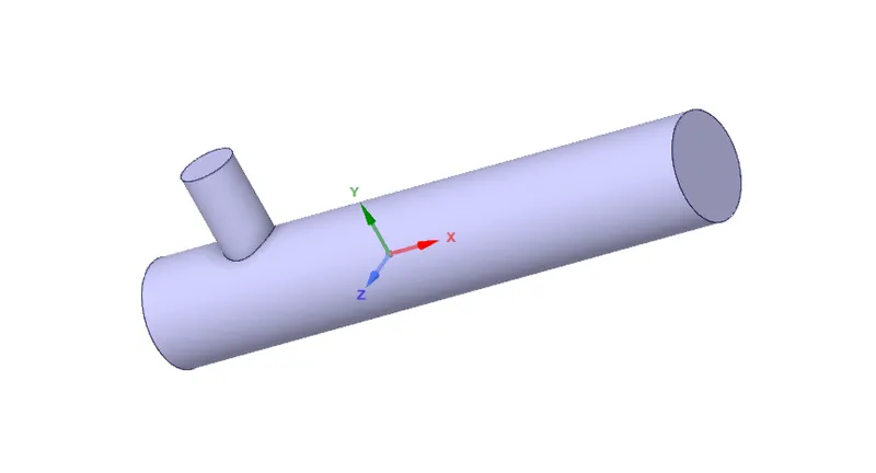
MESHING, this app allows us to generate mesh on the geometry and we also use this app to name and identify boundaries, inlets, outlets, if any.

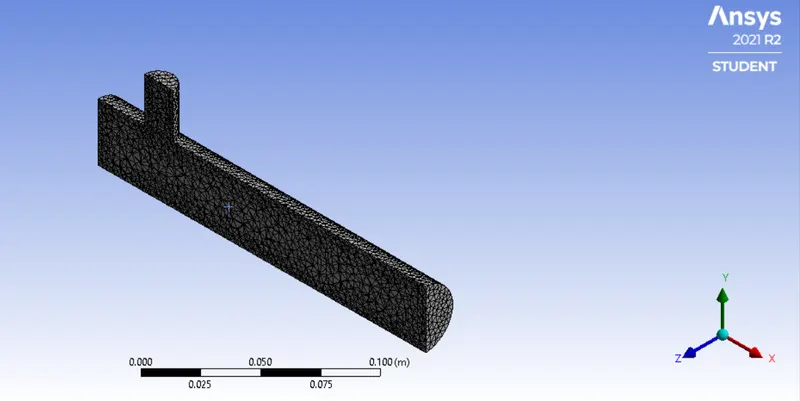
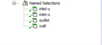
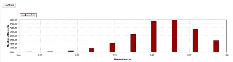
The element size is maintained at 3e-3 due to system limitations.

Setup, in this app we apply different boundary conditions, we assign different roles to different profiles. We chose an appropriate turbulence model (K-ε or K-Ω) for solving the turbulent mixing of the air. This app also allows us to decide the number of iterations that are maintained up to 300 iterations due to system limitations.

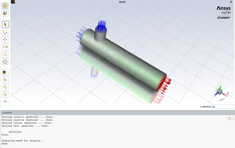
Post-Processing, in this we assign physical properties to the system and set up different contours to visualize the properties.

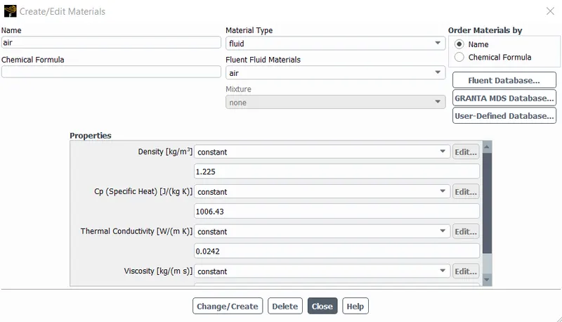
Material properties are assigned (air is the working fluid),

We then assign boundary properties,

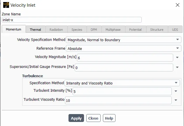
Warm inlet velocity,

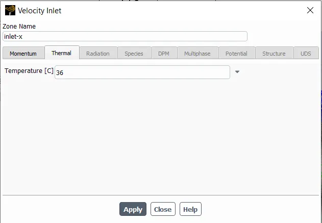
Warm inlet temperature,

The same is done for the properties at the cold inlet.

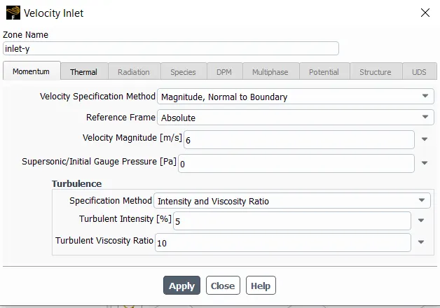
Cold inlet velocity,

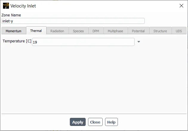
Cold inlet temperature,

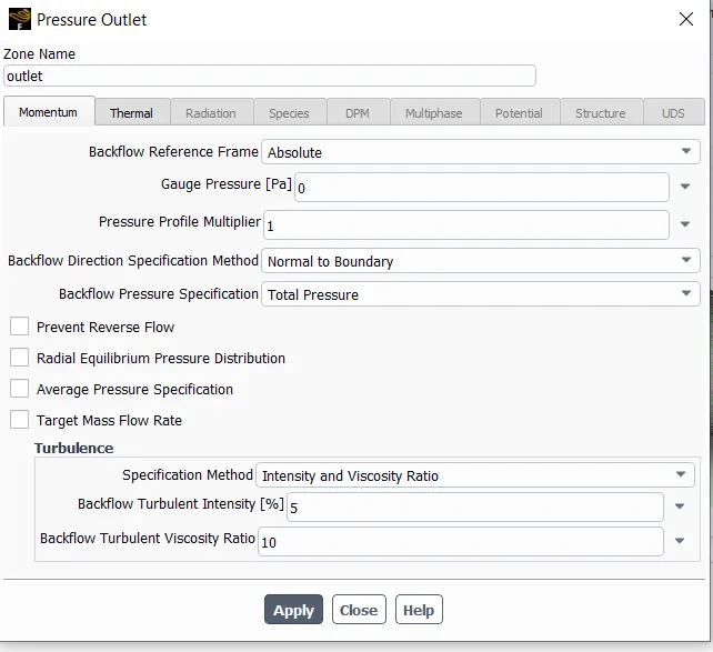
The outlet conditions are also specified and the gauge pressure is maintained at ‘0’ at the outlet.

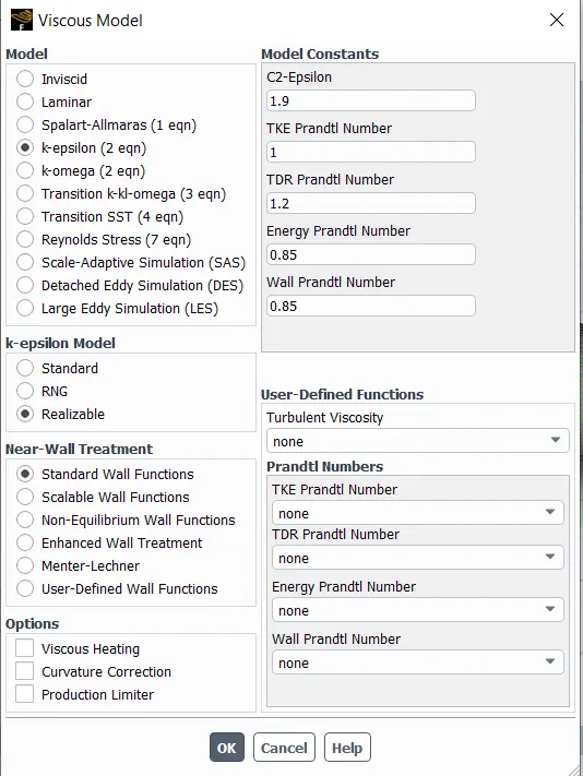
Turbulence model properties are also chosen in this section. The K-ε model (Realisable) is chosen.

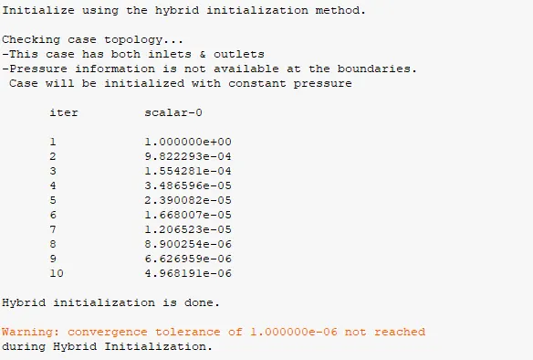
The model is then ‘Initialised’. Doing so all the properties and the flow is brought to the initial condition at time t= 0.

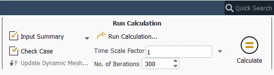
Then we determine the number of desired iterations according to the resources available, for the following simulation we will limit the number of iteration to 300.

With this, the simulation is prepared to run and we generate the results.

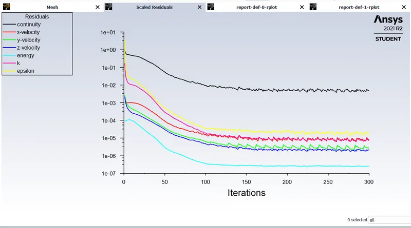
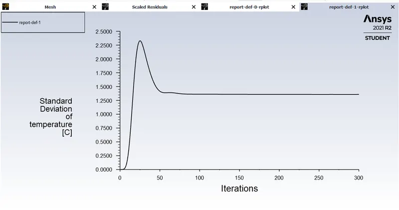
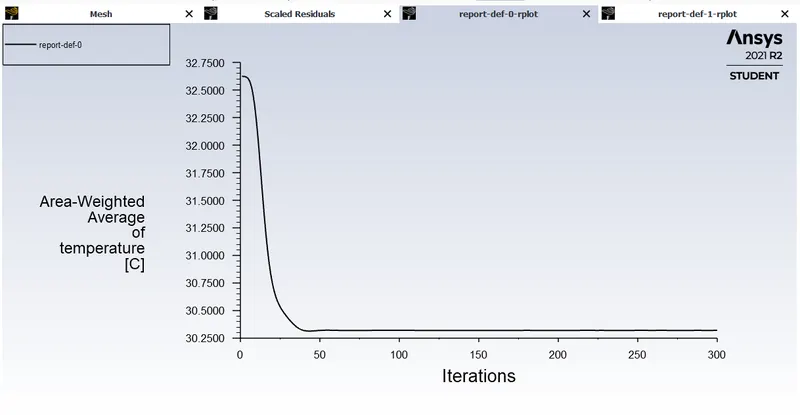
Conclusion, we will get the visual representation of the above simulation in the form of a contour graph and we will generate one for temperature and the second for velocity.

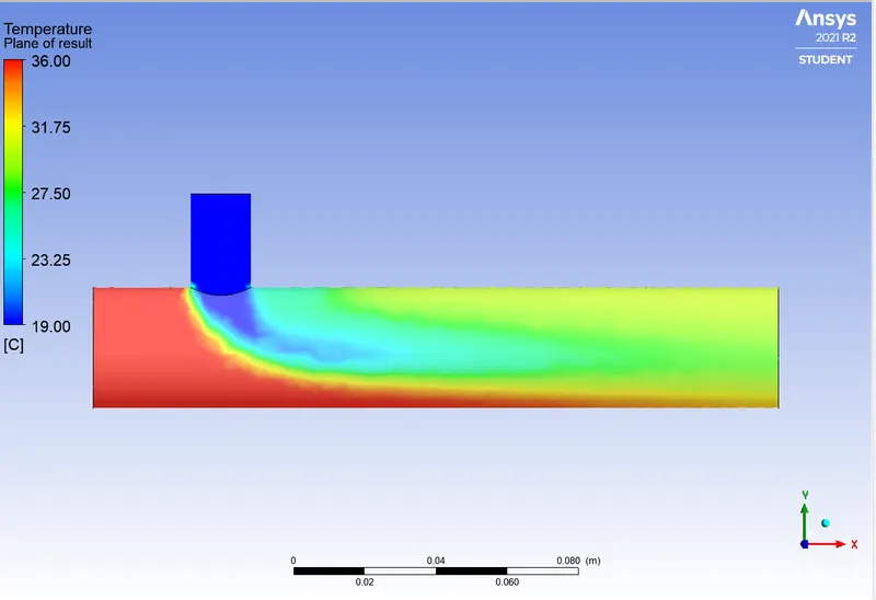
Temperature Contour,

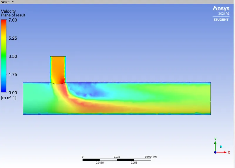
Velocity contour,

Short Tee, Momentum Ratio 4;

For the attempt with the motion ratio increased to 4 we will keep most of the conditions related to the geometry identical, the inputs for the boundaries, inlet, outlet will remain the same. We will change the inlet velocities of the hot and cold air.

In the Fluent app, we will edit the boundaries of the inlets and the outlet and change the velocities for the inlet cold air.

Doing so will change the contour for temperature and the velocities drastically.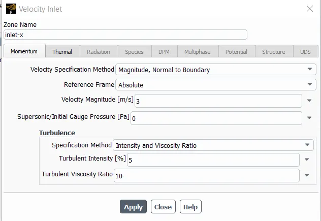

Warm inlet velocity,

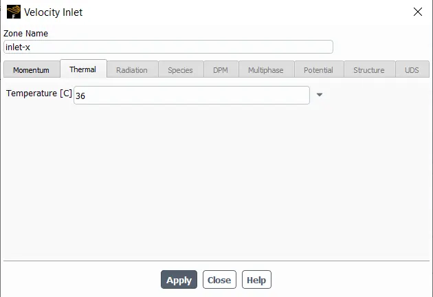
Warm inlet temperature,

The same is done for the properties at the cold inlet.

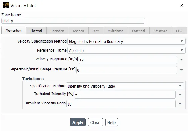
Cold Inlet Velocity,

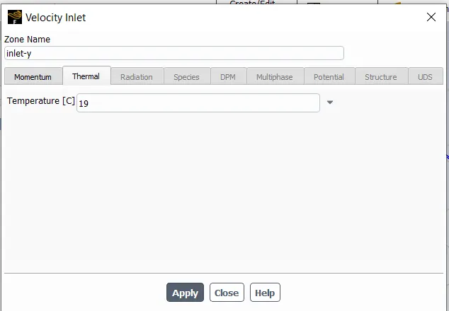
Cold inlet temperature,

The outlet properties will remain the same, we will also keep the Turbulence model the same.

Then we initialise the model and then run the simulation.

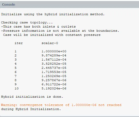
Then we determine the number of desired iterations according to the resources available, for the following simulation we will limit the number of iteration to 300.

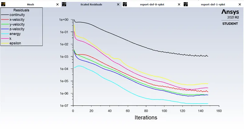
Scalar Residuals

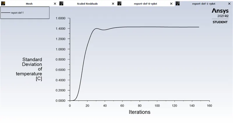
Standard Deviations of temperature,

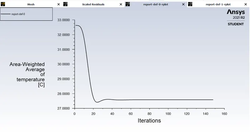
Area weighted average of temperature,

Conclusion, we will get the visual representation of the above simulation in the form of a contour graph and we will generate one for temperature and the second for velocity.

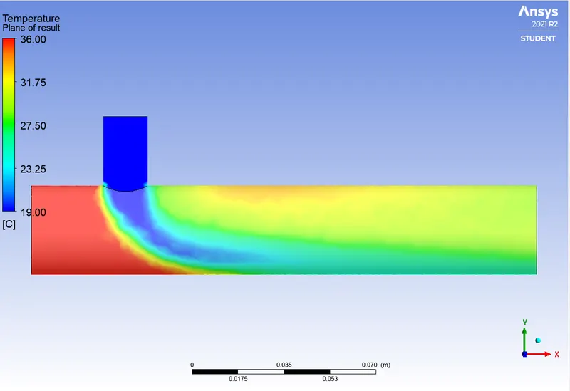
Temperature contour,

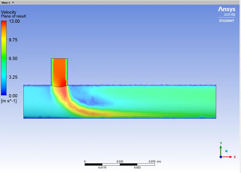
Velocity Contour,

Long Tee, Momentum Ratio 2;

CAD Cleanup with SpaceClean, this app is used to clean the generated model and get the relevant volume from the model.

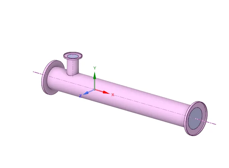
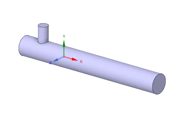
MESHING, this app allows us to generate mesh on the geometry and we also use this app to name and identify boundaries, inlets, outlets, if any.

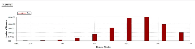
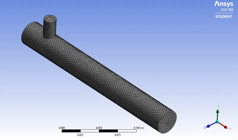
The element size is maintained at 3e-3 due to system limitations.

Setup, in this app we apply different boundary conditions, we assign different roles to different profiles. We chose an appropriate turbulence model (K-ε or K-Ω) for solving the turbulent mixing of the air. This app also allows us to decide the number of iterations that are maintained up toinitialize300 iterations due to system limitations.

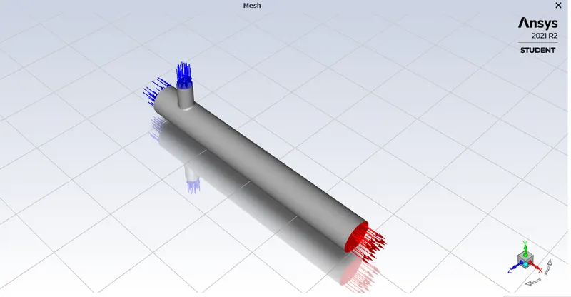
Post-Processing, in this we assign physical properties to the system and set up different contours to visualize the properties.

Material properties are assigned (air is the working fluid),

We then assign boundary properties,

Cold inlet Velocity

Cold Inlet Temperature

Warm inlet Velocity

Warm inlet temperature

The outlet conditions are also specified and the gauge pressure is maintained at ‘0’ at the outlet.

Turbulence model properties are also chosen in this section. The K-ε model (Realisable) is chosen.

The model is then ‘Initialised’. Doing so all the properties and the flow is brought to the initial condition at time t= 0.

Then we determine the number of desired iterations according to the resources available, for the following simulation we will limit the number of iteration to 300.

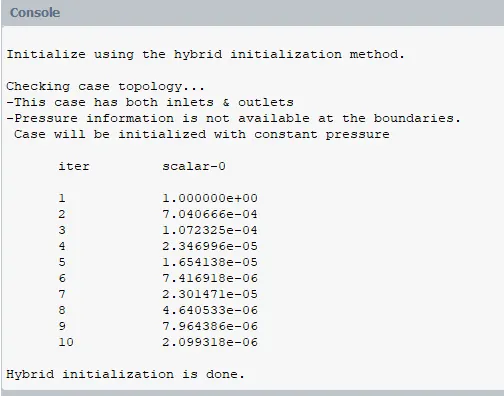
With this, the simulation is prepared to run and we generate the results.

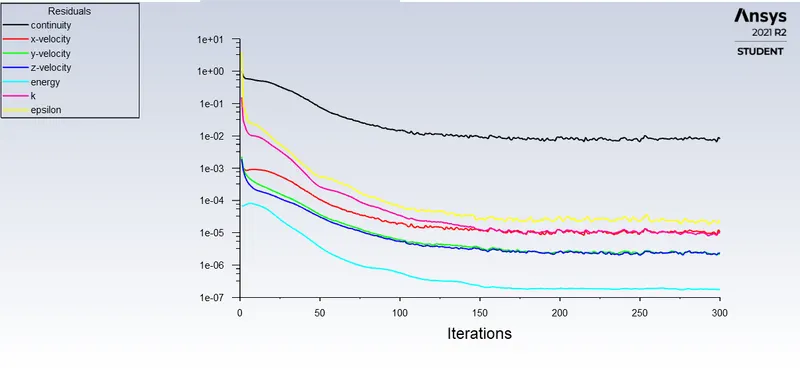
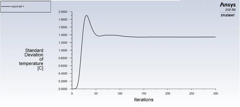
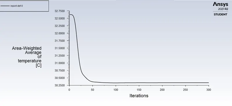
Conclusion, we will get the visual representation of the above simulation in the form of a contour graph and we will generate one for temperature and the second for velocity.

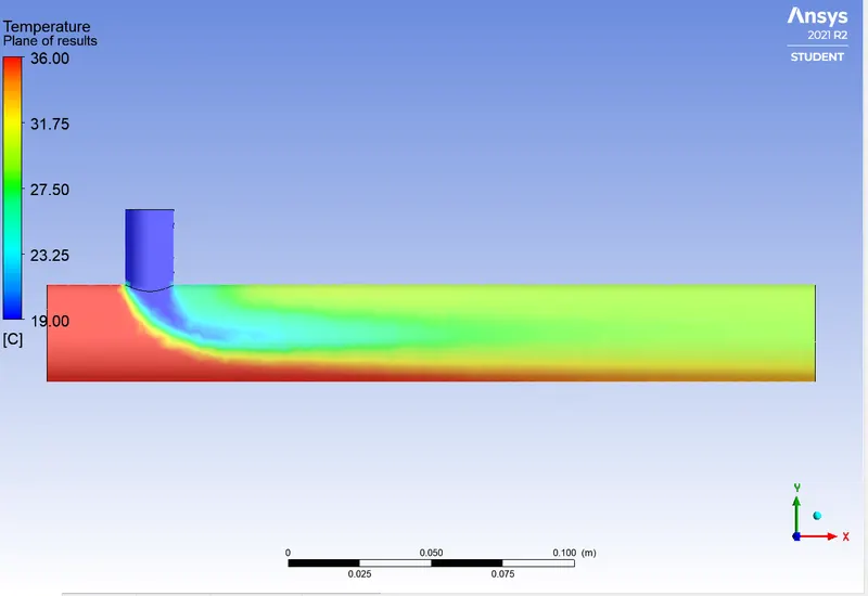
Temperature Contour,

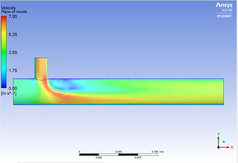
Velocity Contour,

Long Tee, Momentum Ratio 4;

For the attempt with the motion ratio increased to 4 we will keep most of the conditions related to the geometry identical, the inputs for the boundaries, inlet, outlet will remain the same. We will change the inlet velocities of the hot and cold air.

In the Fluent app, we will edit the boundaries of the inlets and the outlet and change the velocities for the inlet cold air.

Doing so will change the contour for temperature and the velocities drastically.

Warm inlet velocity,

Warm inlet temperature,

Cold inlet velocity

Cold inlet temperature,

The outlet properties will remain the same, we will also keep the Turbulence model the same.

Then we initialize the model and then run the simulation.

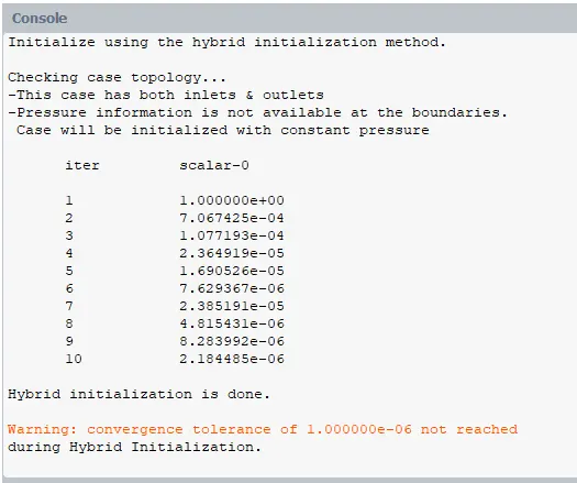
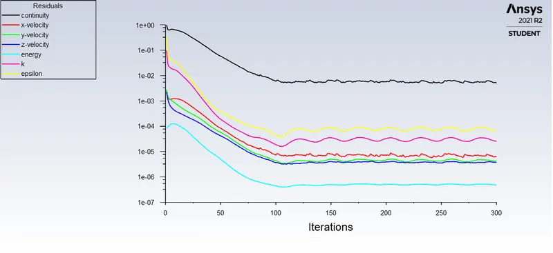
Then we determine the number of desired iterations according to the resources available, for the following simulation we will limit the number of iteration to 300.

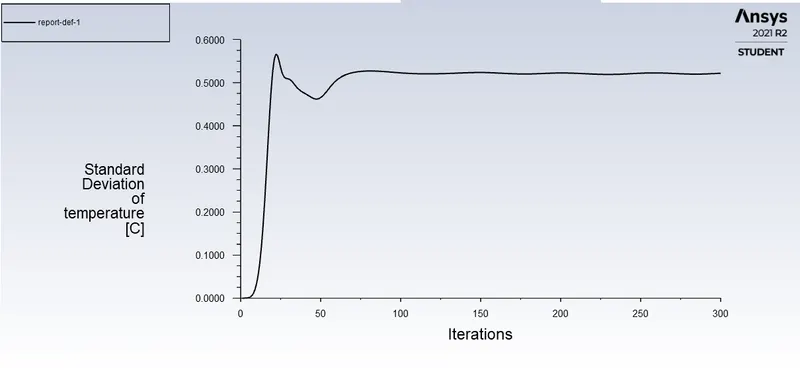
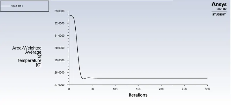
Conclusion, we will get the visual representation of the above simulation in the form of a contour graph and we will generate one for temperature and the second for velocity.

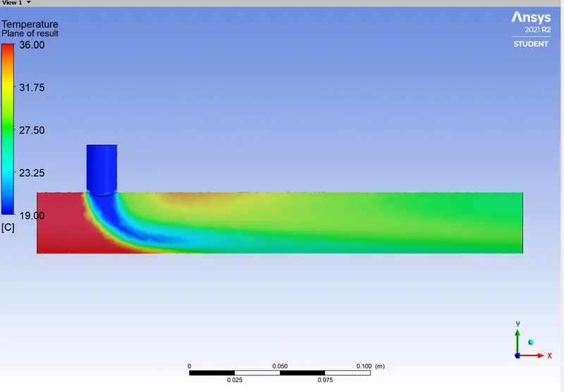
Temperature Contour,

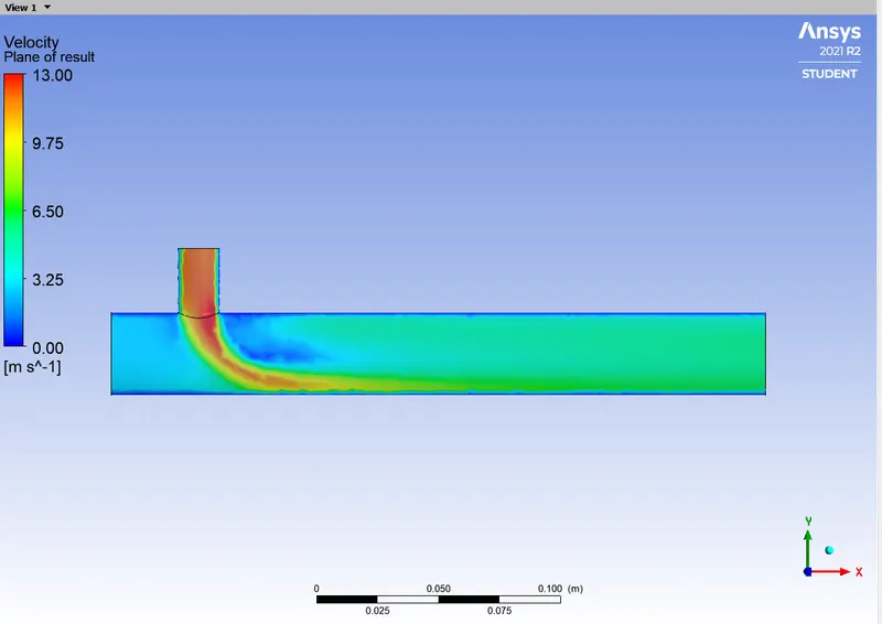
Velocity Contour.

Conclusion

• As we observe that the temperature at the outlet drops down considerably when the momentum ratio is 4.
• This is due to increased turbulent mixing at the tee joint between hot air and cold air because of the high velocity of the cold air. This is why the temperature drop in low momentum ratio models is not as much as the higher momentum ratio model irrespective of the length.
• In the shorter tee model, we can observe that the mixing of hot and cold air is not that efficient, on the other hand in the case of the long tee model the mixing is comparatively more efficient.
• So, with these results, we can conclude that the long-tee with high momentum ratio should be preferred. We can also say that the long teeth have a low standard deviation compared to the short tee for either of the momentum ratios.
• K-ϵ is usually preferred as a standard since it predicts turbulence away from the boundary. On the other hand, the K-Ω model does so near the boundary. Since our concern was the floor away from the wall we used the K-ϵ model for the turbulence rather than the K-Ω model.

Report Link: https://docs.google.com/document/d/1eR91zluuFvZ0TbW2Q-yE7iDXtJ45dKIXUO7KwP_X53o/edit?usp=sharing