Week 11 - Simulation of Flow through a pipe in OpenFoam
Flow-Through a Pipe
Simulation Through OpenFoam
Introduction
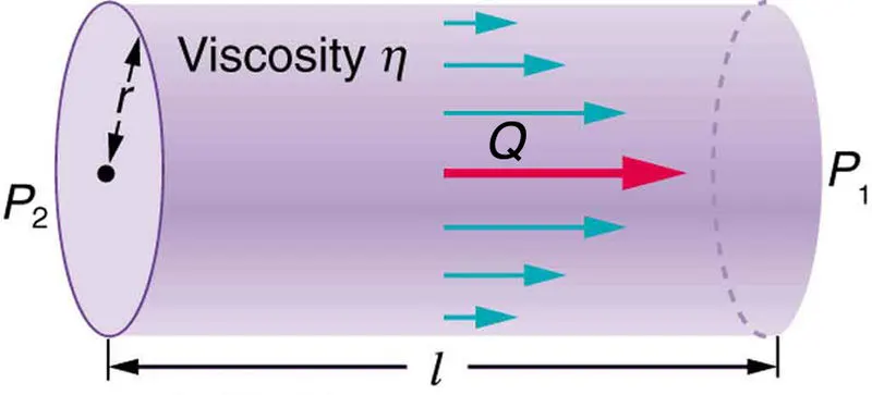
Flow-through a pipe or in this case The Hagen Poiseuille's Flow, laminar flow occurring in a smooth cylindrical pipe.
Internal flow through a pipe is the common flow example. In the case of laminar flow, we consider layers of fluid sliding over each other in the direction parallel to their plane. The layer of fluid in contact with the wall of the pipe is at complete rest i.e. no-slip condition. Starting from the wall we move in the radial direction to the centre of the pipe velocity keeps increasing.
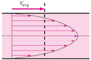
This problem is a perfect example of a parabolic partial differential equation. When we compare the layers of fluid moving relative to each other the layer just above is moving faster than the layer below it, and the layer just below is moving slower than the layer above it, because of this the layer above pushes the layer just below it in forwarding direction and the layer below pulls the layer above backward. This force generates shear stress in the layer. As all the layers have velocities relative to each other, drag is generated amongst them.
The layer of fluid at the wall/ boundary has zero velocity e but the highest shear stress. The shear stress at the centre is the lowest and speed is the highest.
When the fluid starts flowing in the pipe we consider a hypothetical boundary layer, as the fluid enters the pipe the boundary thickens as the fluid reaches 99% of free stream velocity. This is called the boundary layer.
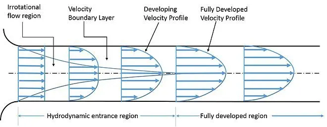
The velocity profile is parabolic but the fluid attains the parabolic profile only when it has achieved the free stream and stability. Initially, the floor is not stable as it enters the pipe and after travelling some distance it does so, the distance the fluid has to travel from entry of the pipe to the point at developing/stabilize is called hydrodynamic entry length.
It can also be said as the length of the entrance is the distance that fluid travels after entering a pipe before the full development of the flow. Entrance length refers to the length of the entry region where effects from the pipe interior wall spread as an expanding boundary layer into the flow. When the boundary layer extends to fill the entire pipe the flow grows into a fully developed flow where the flow characteristics no longer change with increased distance along the pipe.
The hydrodynamic entrance region is an area of the pipe where the fluid entering the pipe develops a viscous force spreading from the pipes’ interior wall. Non-uniform flow is observed in this region; the velocity of fluid entering the pipe is constant but the fluid at the boundary/wall is stationary.
The layer in contact with the surface is affected by the acceleration of the neighbouring layers due to viscous force within the fluid acting as friction and slowing the adjacent layers this Den rate the velocity profile and keep the mass flow rate conserved therefore the speed at the centre of the pipe increases as a compensation. This effect is the reason for the creation of velocity gradient and velocity profile.
Problem
Simulation of flow through the pipe in OpenFoam.
- Calculation of flow variables.
- Generation of blockMeshDict using wedge boundary condition.
- Create the blockMeshDict file in MATLAB such that the mesh is automatically created with the wedge angles.
- Simulate the pipe flow in OpenFoam using icoFoam solver.
- Post-process the velocity profile and shear stress and compare the results of the simulation with analytical results obtained using Hagen Poiseuille's equation.
Assumptions
- The fluid obeys Newton's law of viscosity.
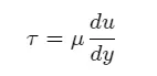
- No-slip of fluid particles at the boundary.
Flow Variables
Working fluid is water,
- Density (ρ) = 1000kg/m^3
- Dynamic viscosity (μ) = 8.90 x 10^(-4) pa.s
- Reynolds number (Re) = 2100
- Diameter of the pipe (D) = 0.004 m
Formulas and Calculations
- Hydrodynamic entry length is calculated using a formula,
- Laminar flow; Lh = 0.05* Re*D
- Turbulent flow; Lh = 1.359*D*(Re)1/4
- Lh = Hydrodynamic Length
- Re = Reynolds number
- D = characteristic length (or diameter)
- Hagen Poiseuille's Law: In non-ideal fluid dynamics Hagen Poiseuille equation is a physical law that gives pressure drop in an incompressible and Newtonian fluid in a laminar flow through a long cylindrical pipe of constant cross-section.
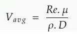
- Average velocity (V_avg)
- Max velocity (V_max)
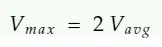
- Max velocity (V_max)
-
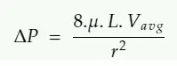
- Pressure Difference (ΔP)
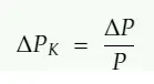
- The kinematic pressure difference (ΔPK)
- Shear stress (τ)
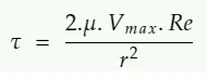
- V(r) = Vmax(R2 - r2)/R2
Computation
First, we use MATLAB to compute the solution and solve for the variables and also to generate the files to be post-processed in OpenFoam.
- Pressure Difference (ΔP)
- Average velocity (V_avg)
clear all
close all
clc

%% Inputs
% Renolds Number
Re = 2100;
% Diameter of Pipe
D = 0.04;
% Radius
r = D/2;
% Hydrodynamic entery length
% L = 0.006*Re*D
L = 0.06*Re*D;
% Total Length of Pipe
L_p = L + 0.7;
% Angle of Wedge (less than 5)
theta = 4.5;
% Dynamic Viscocity
mu = 0.89e-3;
% Density
rho = 1000;
%% Hagen Poiseulle Flow Equations
v_avg = (Re*mu)/(rho*D);
v_max = 2*(v_avg);
del_p = (8*mu*L_p*v_avg)/(r^2);
kin_p = del_p/rho;
%% Calculating for tau
R = linspace(0,r,1000);
for i = 1:length(R)
    tau(i) = 2*mu*v_max*(abs(R(i)))/r^2;
end
plot(R,tau)
xlabel('Radius')
ylabel('Shear Stress')
grid on
legend('Shear Stress')

%% File Generation
% Header

header1 = '/*---------------------------------*- C++ -*---------------------------------*\'
header2 = '   =========                 |                                                 '
header3 = '   \\      /  F ield         | OpenFOAM: THe Open Source CFD Toolbox           '
header4 = '    \\    /   O peration     | Website:  https://openfoam.org                  '
header5 = '     \\  /    A nd           | Version:  7                                     '
header6 = '      \\/     M anipulation  |                                                 '
header7 = '\*---------------------------------------------------------------------------*/'

f1 = fopen('blockMeshDict','w')
fprintf(f1, '%s\n', header1)
fprintf(f1, '%s\n', header2)
fprintf(f1, '%s\n', header3)
fprintf(f1, '%s\n', header4)
fprintf(f1, '%s\n', header5)
fprintf(f1, '%s\n', header6)
fprintf(f1, '%s\n', header7)

fprintf(f1, 'FoamFile\n{\n')
fprintf(f1, '%12s \t 2.0;\n','version')
fprintf(f1, '%11s  \t ascii;\n','format')
fprintf(f1, '%10s \t\t dictionary;\n','class')
fprintf(f1, '%11s  \t blockMeshDict;\n','object')
fprintf(f1, '}\n')
header8 = '// * * * * * * * * * * * * * * * * * * * * * * * * * * * * * * * * * * * * * //'
fprintf(f1, '%s\n\n',header8)

fprintf(f1, 'convertToMeters 1;\n\n')

fprintf(f1, 'vertices\n')
fprintf(f1, '(\n')
fprintf(f1, '\t (%d %d %d)\n',0,0,0)
fprintf(f1, '\t (%d %d %d)\n',0,r*cosd(theta/2),r*sind(theta/2))
fprintf(f1, '\t (%d %d %d)\n',0,r*cosd(theta/2),-r*sind(theta/2))
fprintf(f1, '\t (%d %d %d)\n',L_p,0,0)
fprintf(f1, '\t (%d %d %d)\n',L_p,r*cosd(theta/2),r*sind(theta/2))
fprintf(f1, '\t (%d %d %d)\n',L_p,r*cosd(theta/2),-r*sind(theta/2))
fprintf(f1, ');\n\n')

fprintf(f1, 'blocks\n')
fprintf(f1, '(\n')
fprintf(f1, '\t hex (0 3 5 2 0 3 4 1) (%d %d %d)', 300,30,1)
fprintf(f1, ' SimpleGrading (1 0.1 1)\n\n')
fprintf(f1, ');\n\n')

fprintf(f1, 'edges\n')
fprintf(f1, '(\n')
fprintf(f1, '\t arc %d %d (%d %d %d)\n',1,2,0,r,0)
fprintf(f1, '\t arc %d %d (%d %d %d)\n',4,5,L_p,r,0)
fprintf(f1, ');\n\n')

fprintf(f1, 'boundary\n')
fprintf(f1, '(\n')
fprintf(f1, '\t inlet \n')
fprintf(f1, '\t {\n')
fprintf(f1, '\t\t type patch;\n')
fprintf(f1, '\t\t faces\n')
fprintf(f1, '\t\t (\n')
fprintf(f1, '\t\t\t (0 1 2 0)\n')
fprintf(f1, '\t\t );\n')
fprintf(f1, '\t }\n')

fprintf(f1, '\t outlet\n')
fprintf(f1, '\t {\n')
fprintf(f1, '\t\t type patch;\n')
fprintf(f1, '\t\t faces\n')
fprintf(f1, '\t\t (\n')
fprintf(f1, '\t\t\t (3 5 4 3)\n')
fprintf(f1, '\t\t );\n')
fprintf(f1, '\t }\n')

fprintf(f1, '\t top\n')
fprintf(f1, '\t {\n')
fprintf(f1, '\t\t type wall;\n')
fprintf(f1, '\t\t faces\n')
fprintf(f1, '\t\t (\n')
fprintf(f1, '\t\t\t (1 4 5 2)\n')
fprintf(f1, '\t\t );\n')
fprintf(f1, '\t }\n')

fprintf(f1, '\t front\n')
fprintf(f1, '\t {\n')
fprintf(f1, '\t\t type wedge;\n')
fprintf(f1, '\t\t faces\n')
fprintf(f1, '\t\t (\n')
fprintf(f1, '\t\t\t (0 3 4 1)\n')
fprintf(f1, '\t\t );\n')
fprintf(f1, '\t }\n')

fprintf(f1, '\t back\n')
fprintf(f1, '\t {\n')
fprintf(f1, '\t\t type wedge;\n')
fprintf(f1, '\t\t faces\n')
fprintf(f1, '\t\t (\n')
fprintf(f1, '\t\t\t (0 2 5 3)\n')
fprintf(f1, '\t\t );\n')
fprintf(f1, '\t }\n')

fprintf(f1, '\t axis\n')
fprintf(f1, '\t {\n')
fprintf(f1, '\t\t type empty;\n')
fprintf(f1, '\t\t faces\n')
fprintf(f1, '\t\t (\n')
fprintf(f1, '\t\t\t (0 3 3 0)\n')
fprintf(f1, '\t\t );\n')
fprintf(f1, '\t }\n')
fprintf(f1, '); \n\n')

fprintf(f1, 'mergePatchPairs\n')
fprintf(f1, '(\n')
fprintf(f1, ');\n')
header9 = '// * * * * * * * * * * * * * * * * * * * * * * * * * * * * * * * * * * * * * //'
fprintf(f1, '%s\n',header9)

fclose(f1)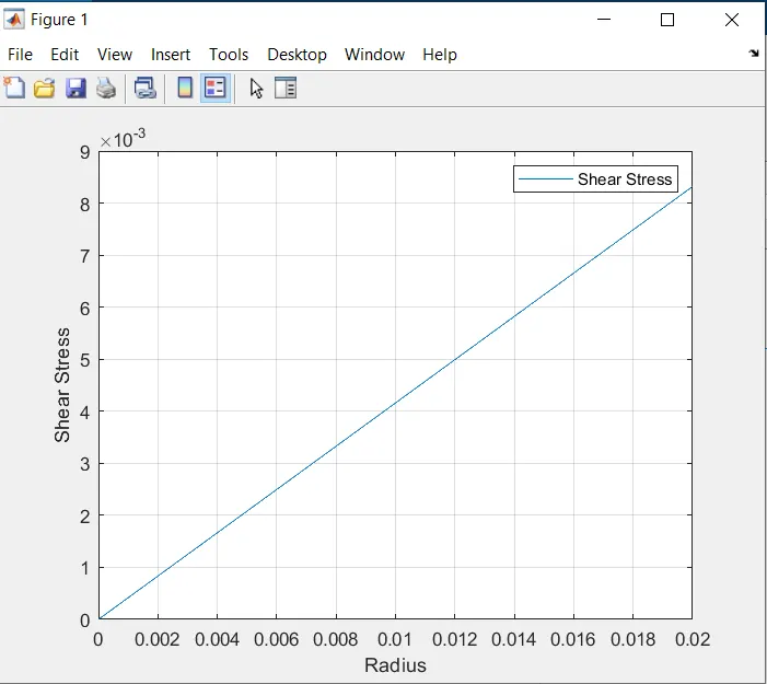
Is the result generated from the Code and also a file is created. blockMeshDict file.
With this, we have generated our ‘blockMeshDict’ file and we will switch to OpenFoam and edit the other files manually.
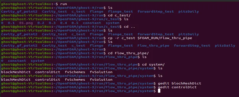
We will start with the ‘blockMeshDict’ file and check the file. Then we will open the ‘controlDict’ file.
BlockMeshDict
/*---------------------------------*- C++ -*---------------------------------*\
   =========                 |
   \\      /  F ield         | OpenFOAM: THe Open Source CFD Toolbox
    \\    /   O peration     | Website:  https://openfoam.org
     \\  /    A nd           | Version:  7
      \\/     M anipulation  |
\*---------------------------------------------------------------------------*/
FoamFile
{
     version 	 2.0;
     format  	 ascii;
     class 	 dictionary;
     object  	 blockMeshDict;
}
// * * * * * * * * * * * * * * * * * * * * * * * * * * * * * * * * * * * * * //

convertToMeters 1;

vertices
(
	 (0 0 0)
	 (0 1.998458e-02 7.851963e-04)
	 (0 1.998458e-02 -7.851963e-04)
	 (5.740000e+00 0 0)
	 (5.740000e+00 1.998458e-02 7.851963e-04)
	 (5.740000e+00 1.998458e-02 -7.851963e-04)
);

blocks
(
	 hex (0 3 5 2 0 3 4 1) (300 30 1) SimpleGrading (1 0.1 1)

);

edges
(
	 arc 1 2 (0 2.000000e-02 0)
	 arc 4 5 (5.740000e+00 2.000000e-02 0)
);

boundary
(
	 inlet
	 {
		 type patch;
		 faces
		 (
			 (0 1 2 0)
		 );
	 }
	 outlet
	 {
		 type patch;
		 faces
		 (
			 (3 5 4 3)
		 );
	 }
	 top
	 {
		 type wall;
		 faces
		 (
			 (1 4 5 2)
		 );
	 }
	 front
	 {
		 type wedge;
		 faces
		 (
			 (0 3 4 1)
		 );
	 }
	 back
	 {
		 type wedge;
		 faces
		 (
			 (0 2 5 3)
		 );
	 }
	 axis
	 {
		 type empty;
		 faces
		 (
			 (0 3 3 0)
		 );
	 }
);

mergePatchPairs
(
);
// * * * * * * * * * * * * * * * * * * * * * * * * * * * * * * * * * * * * * //
ControlDict
/*--------------------------------*- C++ -*----------------------------------*\
  =========                 |
  \\      /  F ield         | OpenFOAM: The Open Source CFD Toolbox
   \\    /   O peration     | Website:  https://openfoam.org
    \\  /    A nd           | Version:  9
     \\/     M anipulation  |
\*---------------------------------------------------------------------------*/
FoamFile
{
    version     2.0;
    format      ascii;
    class       dictionary;
    location    "system";
    object      controlDict;
}
// * * * * * * * * * * * * * * * * * * * * * * * * * * * * * * * * * * * * * //

application     icoFoam;

startFrom       startTime;

startTime       0;

stopAt          endTime;

endTime         50;

deltaT          0.05;

writeControl    timeStep;

writeInterval   50;

purgeWrite      0;

writeFormat     ascii;

writePrecision  6;

writeCompression off;

timeFormat      general;

timePrecision   6;

runTimeModifiable true;


// ************************************************************************* //
After the 'controlDict' file follows the pressure and velocity file in the ‘0’ folder, we make the appropriate changes.
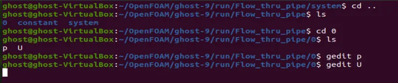
Pressure
/*--------------------------------*- C++ -*----------------------------------*\
  =========                 |
  \\      /  F ield         | OpenFOAM: The Open Source CFD Toolbox
   \\    /   O peration     | Website:  https://openfoam.org
    \\  /    A nd           | Version:  9
     \\/     M anipulation  |
\*---------------------------------------------------------------------------*/
FoamFile
{
    version     2.0;
    format      ascii;
    class       volScalarField;
    object      p;
}
// * * * * * * * * * * * * * * * * * * * * * * * * * * * * * * * * * * * * * //

dimensions      [0 2 -2 0 0 0 0];

internalField   uniform 0;

boundaryField
{
    inlet
    {
        type            zeroGradient;
    }

    outlet
    {
        type            fixedValue;
        value           uniform 0;
    }

    top
    {
        type            zeroGradient;
    }

    front
    {
        type            wedge;
    }

    back
    {
        type            wedge;
    }

    axis
    {
        type            empty;
    }

}

// ************************************************************************* //
Velocity
/*--------------------------------*- C++ -*----------------------------------*\
  =========                 |
  \\      /  F ield         | OpenFOAM: The Open Source CFD Toolbox
   \\    /   O peration     | Website:  https://openfoam.org
    \\  /    A nd           | Version:  9
     \\/     M anipulation  |
\*---------------------------------------------------------------------------*/
FoamFile
{
    version     2.0;
    format      ascii;
    class       volVectorField;
    object      U;
}
// * * * * * * * * * * * * * * * * * * * * * * * * * * * * * * * * * * * * * //

dimensions      [0 1 -1 0 0 0 0];

internalField   uniform (0.0467 0 0);

boundaryField
{
    inlet
    {
        type            fixedValue;
        value           uniform (0.0467 0 0);
    }

    outlet
    {
        type            zeroGradient;
    }

    top
    {
        type            fixedValue;
        value           uniform (0 0 0);
    }

    front
    {
    	type		 wedge;
    }

    back
    {
    	type		 wedge;
    }

    axis
    {
    	type		 empty;
    }

}

// ************************************************************************* //
The ‘transportProperties’ is last.

TransportProperties
/*--------------------------------*- C++ -*----------------------------------*\
  =========                 |
  \\      /  F ield         | OpenFOAM: The Open Source CFD Toolbox
   \\    /   O peration     | Website:  https://openfoam.org
    \\  /    A nd           | Version:  9
     \\/     M anipulation  |
\*---------------------------------------------------------------------------*/
FoamFile
{
    version     2.0;
    format      ascii;
    class       dictionary;
    location    "constant";
    object      transportProperties;
}
// * * * * * * * * * * * * * * * * * * * * * * * * * * * * * * * * * * * * * //

nu              [0 2 -1 0 0 0 0] 8.9256e-07;


// ************************************************************************* //
Conclusion
We then follow the standard procedure of generating mesh using the ‘blockMesh’ command.

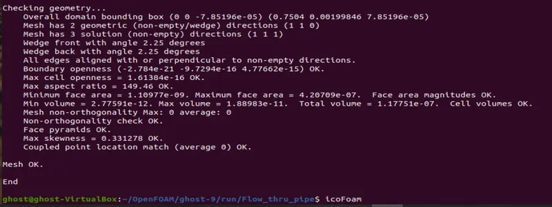
Once we get the mesh we use the ‘checkMesh’ Command.
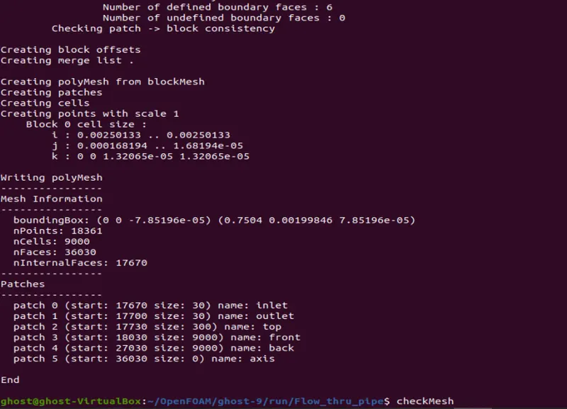
This checks the mesh. And once the output is ‘OK’ we proceed to the icoFoam command to run the simulation.
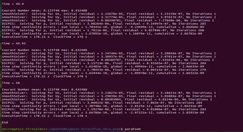
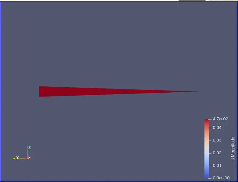
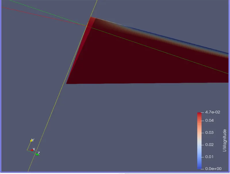
Once we get our results from the ‘icoFoam’ command we use the ‘paraFoam’ command to get the visual representation of the simulation.
Post Processing
We use ParaView to get a visual representation of the flow, in a 3-dimensional space.
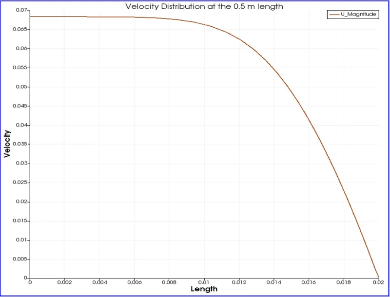
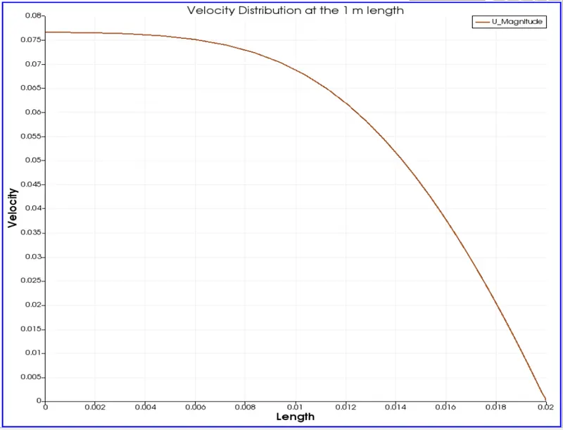
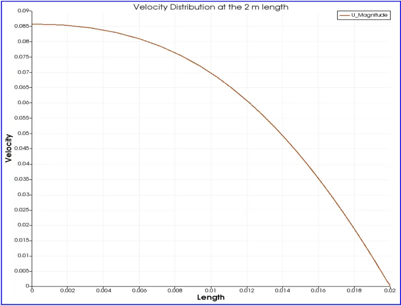
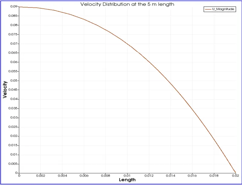
We will use the ‘Plot over line’ command to plot the velocity and pressure curve corresponding to the length of the pipe.
We will start with one end of the pipe (inlet) and check the modifications of the velocity profile across the radial length of the pipe.
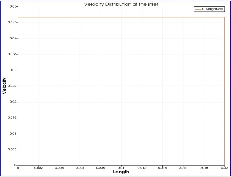
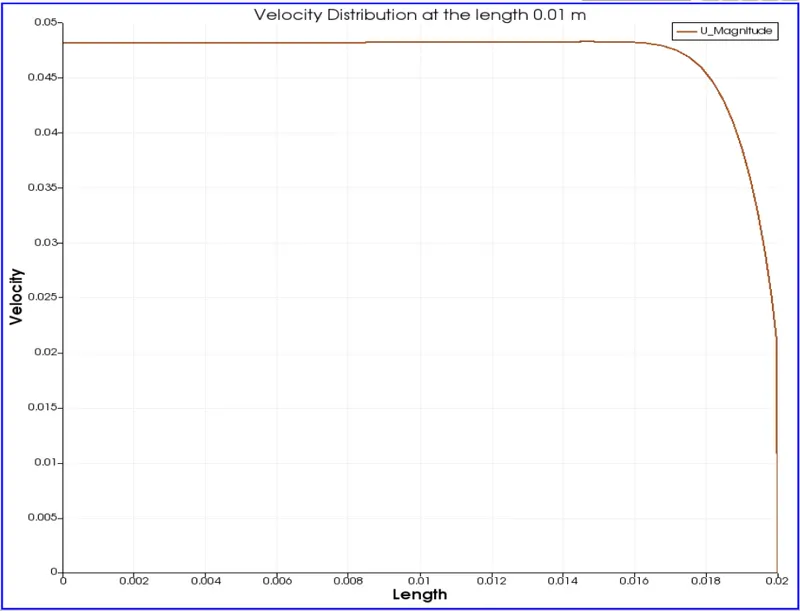
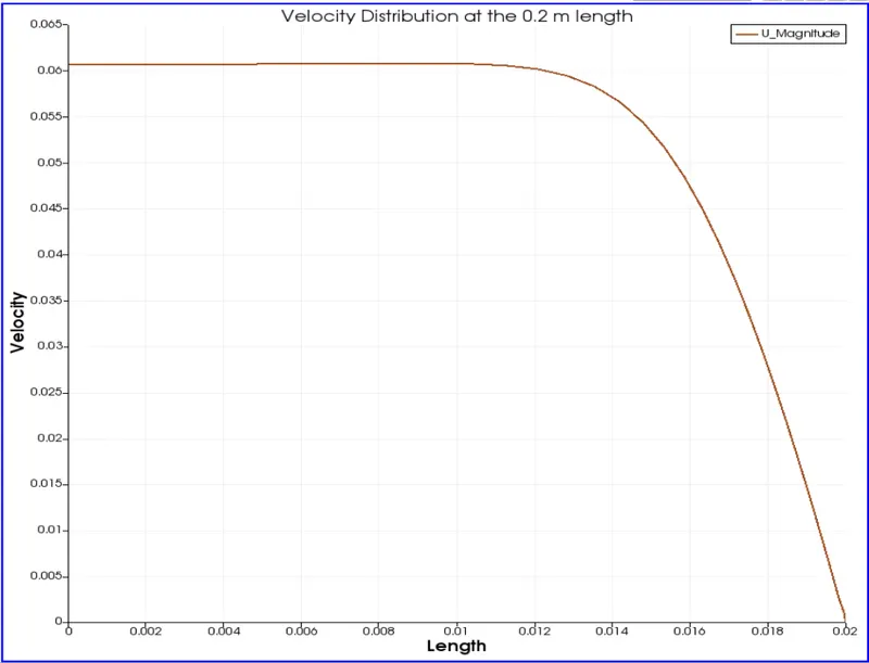
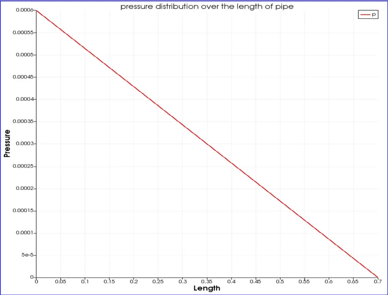
We also need to determine the relation of shear stress and compute the results.
We use MATLAB to generate the code, to compute the relation between the shear stress and radial length.
clear all
close all
clc

%% Input
D = 0.04;
r = D/2;
R = linspace(-0.01,0.01,1000);
Re = 2100;
mu = 8.9e-4;
rho = 1000;
v_avg = (Re*mu)/(rho*D);
v_max = 2*v_avg;

%% Computation
for i = 1:length(R)
    tau(i) = (2*mu*v_max*(abs(R(i))))/(r^2);
end

%% Ploting
figure(1)
plot(R,tau)
xlabel('Radial Distance in "m".')
ylabel('Shear Stress (tau) in N/m^2')
title(sprintf('Change in the Shear Stress for Fully Developed Flow'))
grid minor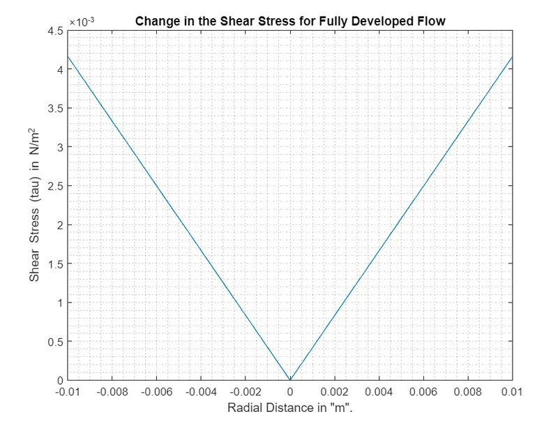
The drawback in the case appears when the Renolds number is large, turbulent flow, after a threshold velocity, for the same geometry the flow transitions from Laminar to turbulent, and the results are rendered unusable.
These results do not work with the turbulent flow because there are no layers to convect. The flow has no order and is unpredictable for the most part.
Report Doc: https://docs.google.com/document/d/18ghxbjwFPsUzf_QenMzJpa5OfH88jJLp-g231u6jZIs/edit?usp=sharing