Simulation of Backward Facing step in the OpenFOAM

Simulation of Incompressible-Laminar-Viscous Flow

Introduction

Before the simulation can be performed we need to elaborate on some concepts, when we talk about the incompressible laminar and viscous flow we are dealing with a Newtonian fluid flowing through a constrained boundary.

Incompressible Flow

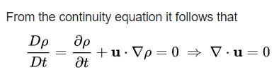
As the name suggests the fluid can’t be compressed and the density remains constant throughout the flow of the fluid.

Dρ/Dt = 0.

Laminar Flow

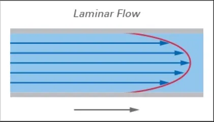
It is a type of flow where the layers of fluid flow over each other parallelly and do not mix amongst each other, this characteristic is observed when the fluid is travelling at a low speed undisturbed and is a perfect example of parabolic PDE. Reynolds number also affects the laminar flow and its transition into turbulent flow.

Viscous Flow

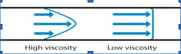
A type of fluid flow in which there is a contentious steady motion of the particles; the motion at a point always remains constant, a flow in which the frictional effect becomes important.

Other important concepts;

Mesh Grading

It is the ratio of the size of the last cell to the size of the first cell, this is the grading factor used substantially in the computation using block mesh.

Problem

Simulate an incompressible-laminar-viscous through the backwards-facing step geometry. Perform the transient simulation.

Case 1: Simulation of the flow without the changes in the default value of the grading factor,

Case 2: Simulate the flow with the grading factor of 0.2, the cells should be finer near the walls.

Solution Without Applying the Grading factor

Mesh Specifications

1. Number of cells along the x directions (longer dimension) = 200,
2. Number of cells along the x directions = 20

Boundary Specifications

The boundary/geometry of the problem is as follows,

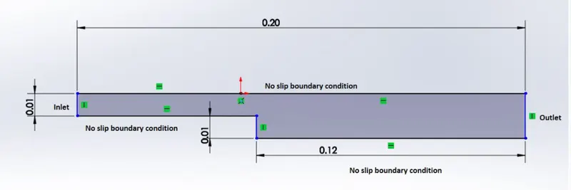
The boundaries are determined within the OpenFOAM software itself,

The terminal is used to navigate in the OpenFOAM (ubuntu)

1. The required file from the tutorial file is copied from the tutorial folder to the RUN folder where we will alter the properties, geometry, and mesh structure according to the requirement.

2. The file required is the ‘cavity’ file, it is copied in the run folder and renamed as ‘Cavity_test’.

3. We now navigate our way to the system folder within the cavity folder as within the cavity folder we have 3 files, ‘0’, ‘constant’, ‘system’.

4. The system folder has 4 files within it, and out of which only 2 files are of concern, the ‘blockMeshDict’, and the ‘controlDict’.

5. With the ‘gedit’ command we will alter the codes of both of these files.

6. BlockMeshDict files allow us to control the geometry and the surfaces concerned, and the 'controlDict' allows us to control time variation.

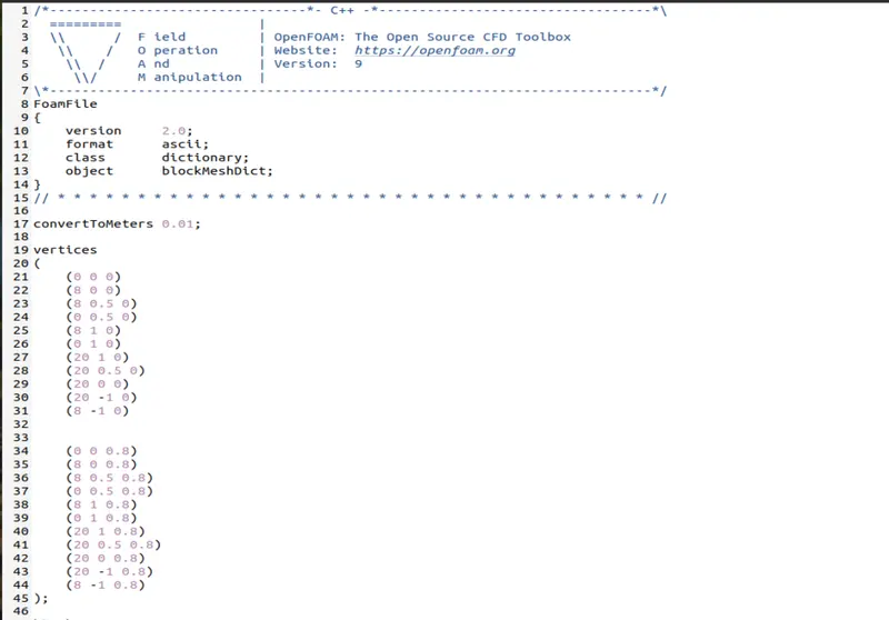
The code here is similar to the codes generated in the C++ language; the header is not read by the solver the ‘FoamFile’ section gives the information about the file/code it is also known as a key-value pair; next follows the convertToMeters command whose function is exactly what it says it is controlling the units of input; the geometry is defined by altering the vertices as shown above.

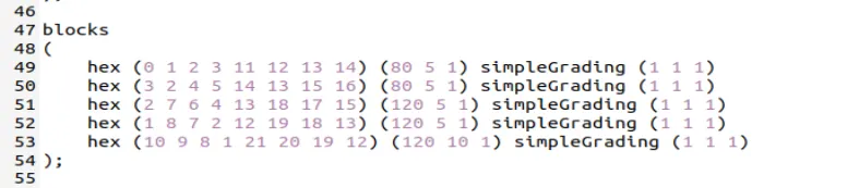
In this part of the code, the ‘hex’ command specifies the type of mesh i.e. hexahedral mesh the units next to it in the 1st bracket specify the block the whole geometry is divided into 5 blocks. Next to the block specifications is grid info, which tells us the number of mesh/nodes will be the volume of concern divided. This is followed by a command ‘simpleGrading command’ whose purpose is to control the size of the mesh within the volume of concern.

What 'simpleGrading' dose is, it uses a factor called a Grading Factor, a.k.a. Expansion ratio which enables the mesh to be graded, or refined in a specified direction. The ratio of the width of the end cell δ, along one edge of the block to the width of the start cell δ.

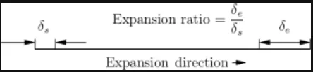
I.e. expansion ratio = (Size of end cell)/(size of starting cell)

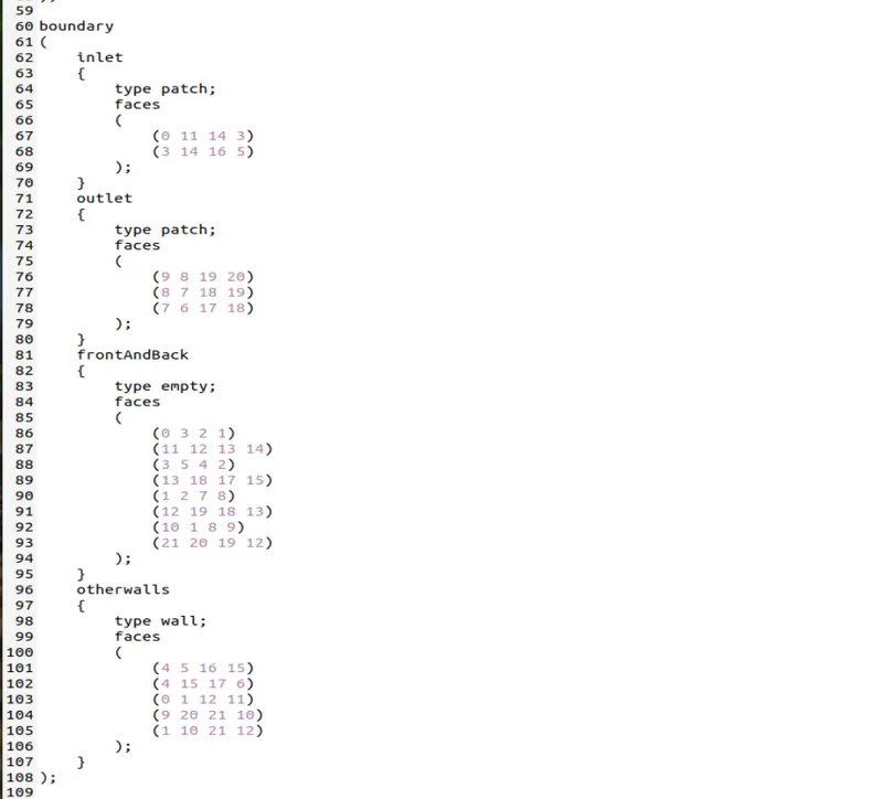
Now lastly this part of the code shows all the walls and the boundaries.

7. After this, the code is saved and closed and we open the 'controlDict' file in the same folder in the same way,

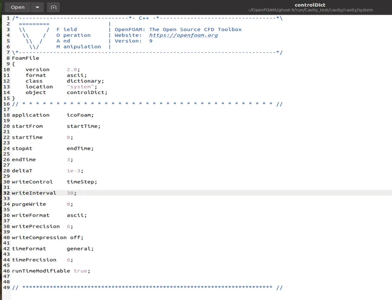
We modify the code by putting in the appropriate value of the ‘endTime’, ‘deltaT’, and ‘writeInterval’, these 3 values play an important role in running the simulation. Then the code is saved and closed.

8. We now navigate our way to the ‘0’ folder which contains the initial value of the pressure and velocity and the code is accessed via the ‘gedit’ command again and in the pressure code, the necessary changes are made corresponding to every type of wall/boundary.

9. The same process is repeated for the velocity file/code: all the units are allotted and the velocity corresponding to each wall/ boundary type is acknowledged and the initial value of the velocity is given.

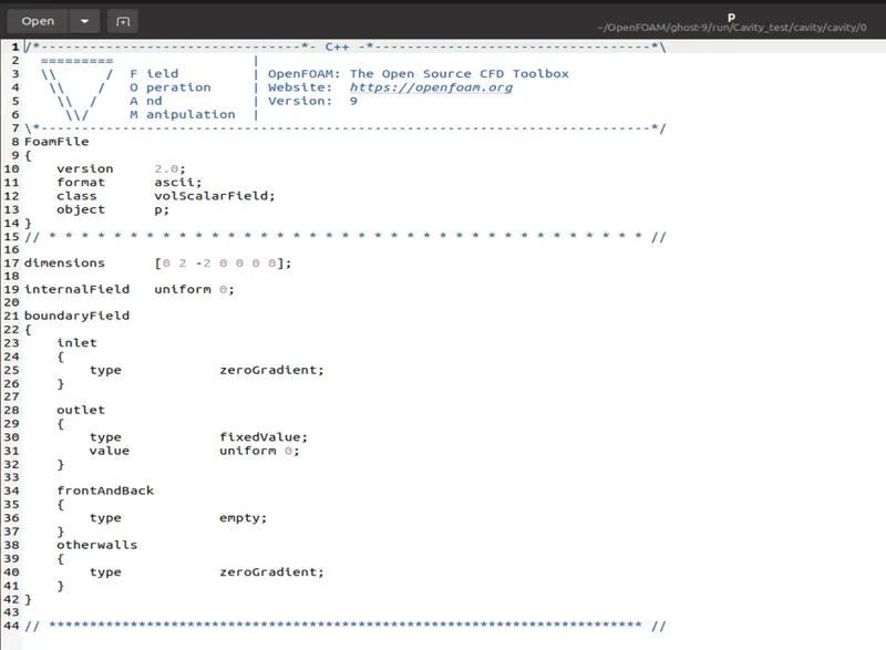
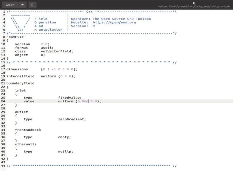
As mentioned we will alter the codes for velocities and the pressure as shown, saved, and closed the codes.

10. Now finally we will go to the ‘constant’ folder and open the ‘transportProperties’ file/code with the ’gedit’ command and make the following changes.

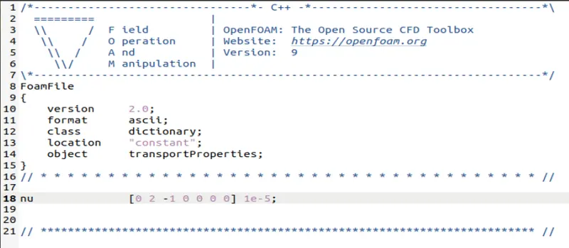
Doing so will change our value of dynamic viscosity.

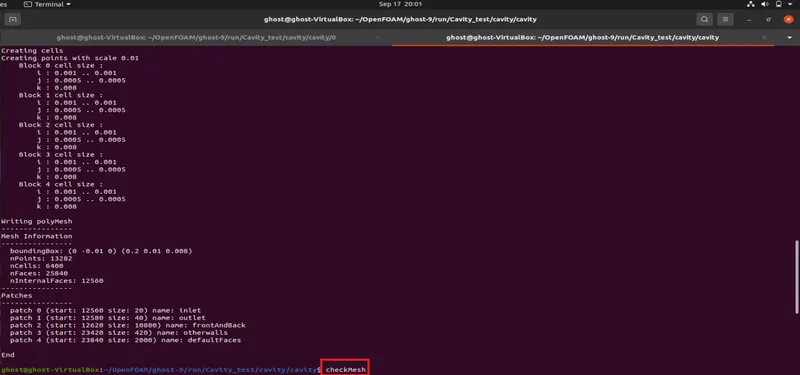
11. Now we will use the ‘blockMesh’ command after returning to the previous folder which will generate the required mesh for us using the ‘blockMeshDict’ file.

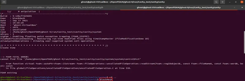
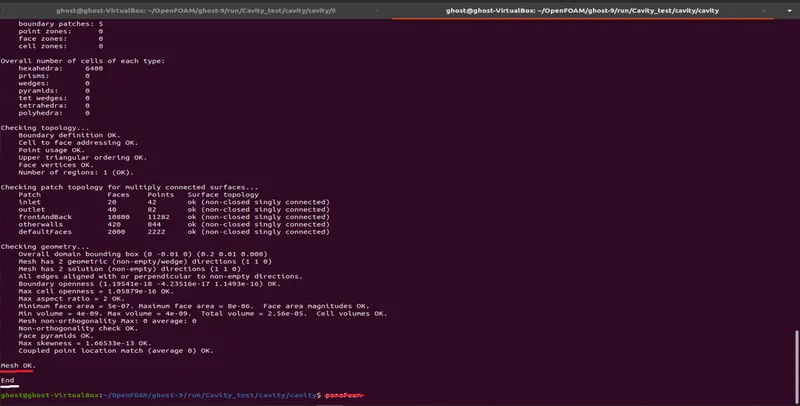
12. When the mesh is generated we use the command ‘checkMesh’ which checks the mesh as the name suggests. And when it gives the signal that the mesh is okay we go ahead and use the ‘icoFoam’ command which runs the simulation and generates the result for each timestep.

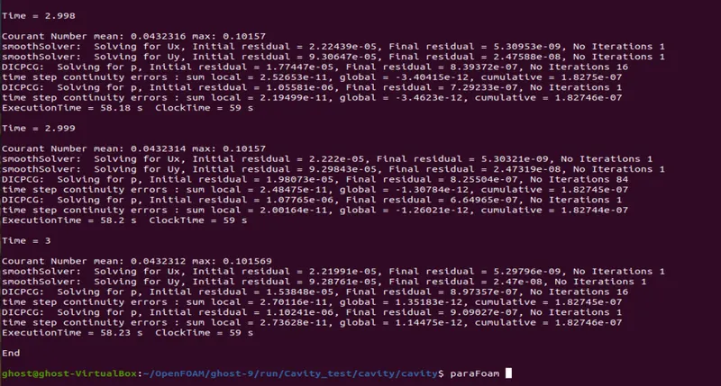
13. Now finally we will run paraFoam to get a visual representation of the results.

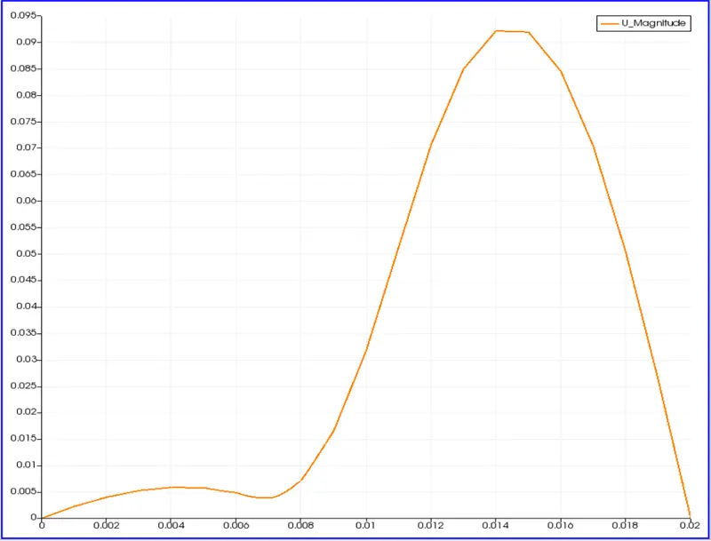
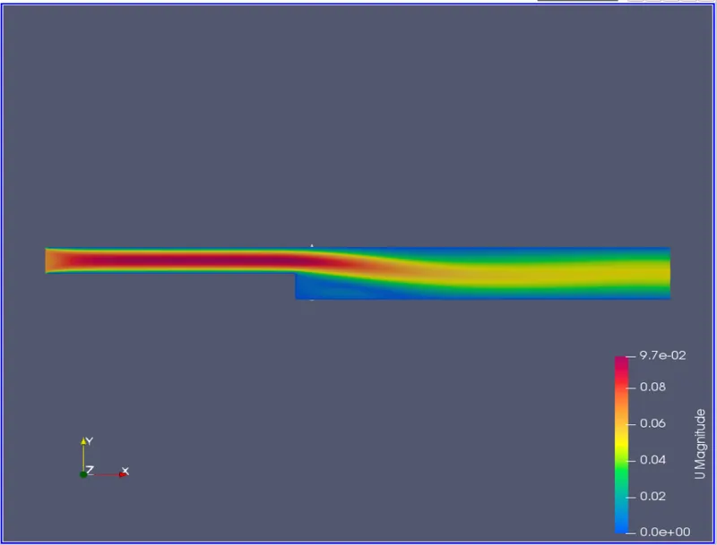
And paraFoam gives us the following results.

And when we run the simulation we get the desired results.

Output: https://drive.google.com/file/d/1tQLyGXI_8FB_gm0n_lSq2i5gYsBCaFiX/view?usp=sharing

Solution After Applying the Grading Factor of 0.2

The majority of the solution and coding will remain the same and the procedure will not change. The changes will appear firstly in the ‘blockMeshDict’ file in the step when we segregate the blocks of the geometry and specify the mesh the ‘simpleGrading’ factors will change accordingly.

The mesh specification will remain the same in terms of the numbers of cells in the ‘x’, ‘y’, and ‘z’ but the size of the cells will change.

The boundary will also remain the same so we can start by duplicating the folder we used above.

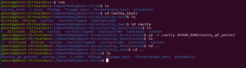
After this, we will navigate our way to the ‘blockMeshDict’ file inside the system folder and access the code via the ‘gedit’ command and make the necessary changes.

In this code, we will alter the ‘simpleGrading’ brackets of the 5 blocks we previously specified.

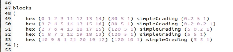
With this step, we have altered the mesh structure and the rest of the code will remain as it is.

We will navigate our way back to the previous folder and use the ’blockMesh’ command and let the solver generate the mesh and geometry according to the codes of the ‘blockMeshDict’ file.

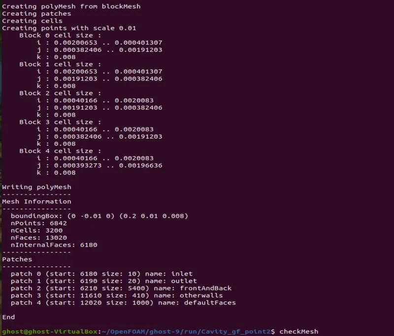
This is then followed by the ‘checkMesh’ command.

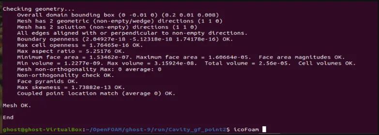
After the approval, we run the ‘icoFoam’ solver/command to start the simulation.

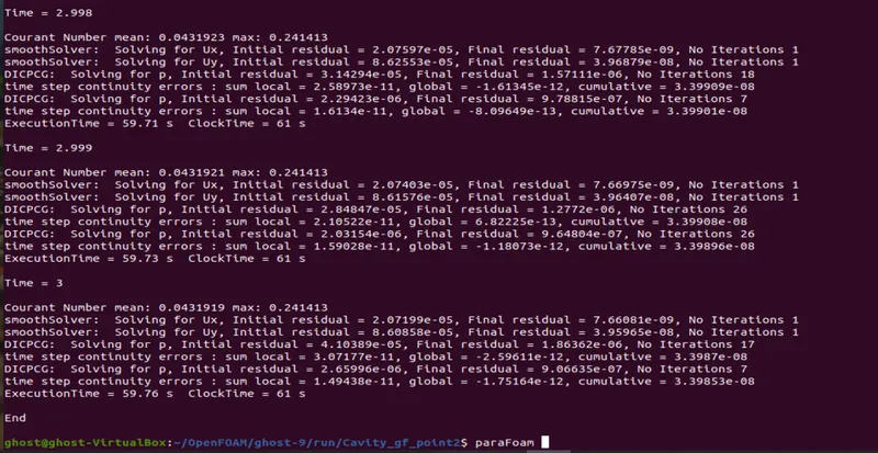
Once this is also done and the results are generated we are free to run ‘paraFoam’ and get a visual representation.

We can see the mesh is concentrated at the centre and the mesh around the inlet and the outlet is less dense and the cell size at the outlet and inlet is more, compared to that of at the middle of the geometry.

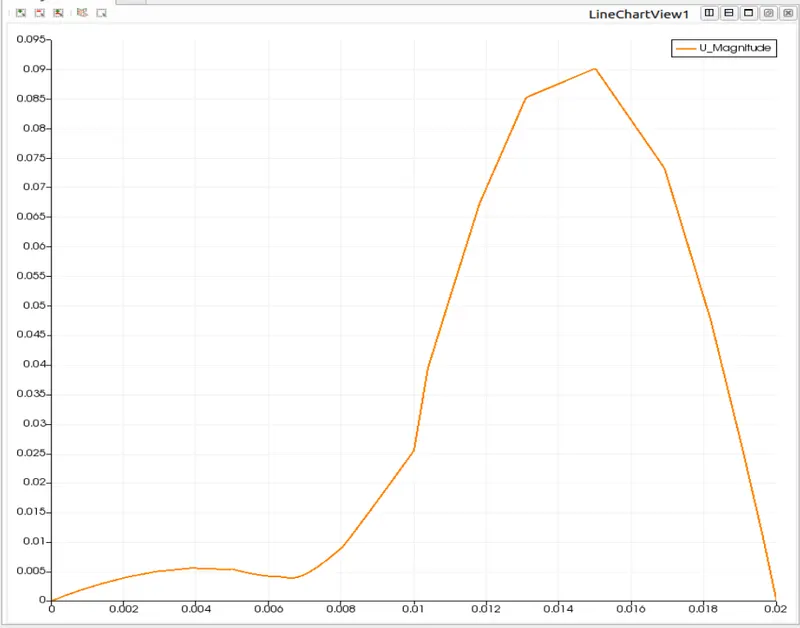
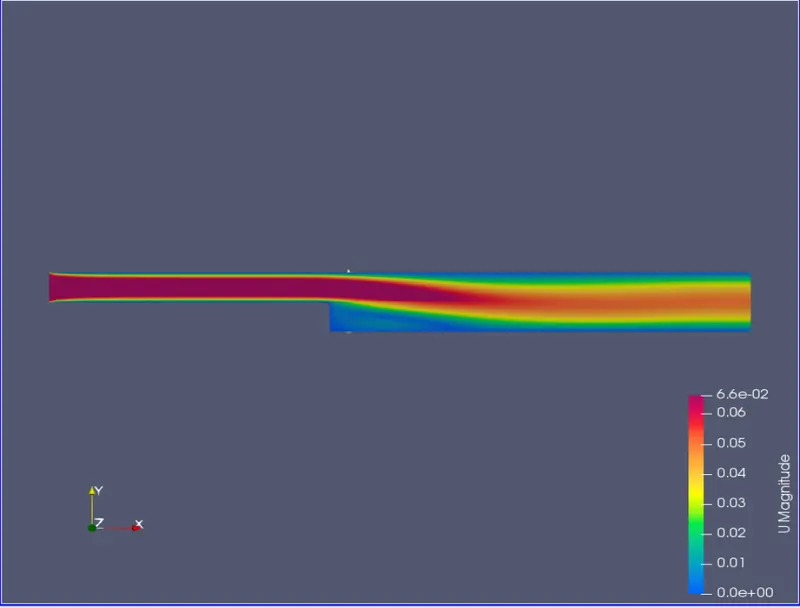
The other physical parameter remained the same and the output is as follows.

Output: https://drive.google.com/file/d/1pIV7fCjXFKF6-80NxhKbXhdP9PXyICu0/view?usp=sharing

Conclusion

Upon changing the grading factor (1 to 0.2) the mesh becomes finer and the solution becomes more accurate. Visually the outputs are similar. Though the computational time was lower for the execution for the lower grading factor.

Report List: https://docs.google.com/document/d/1xomidDbRrLzwHNu-hTesPUvR21sh96A7JjhjejLblyM/edit?usp=sharing