Week 3.5 - Deriving 4th order approximation of a 2nd order derivative using Taylor Table method
Objective To derive the fourth order approximation for the second order derivative by following methods:
- Central difference
- Skewed right side difference
- Skewed left side difference
Taylor table for central difference:

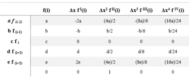
From the above Taylor table, equations extracted are
a + b + c + d + e = 0
-2a-b + d + 2e = 0
4a/2 + b/2 + d/2 + 4e/2 = 1
-8a-b/6 + d/6 + 8e/6 = 0
16a/24 + b/24 + d/24 + 16e/24 = 0
Now we have 5 equations and 5 variables which can be solved in MATLAB program, by which we can obtain a,b,c,d,e which can be solved in central difference approximation.
clc;
clear all;
close all;

% Calculation of central difference coefficients
A = [1 1 1 1 1;-2 -1 0 1 2;2 1/2 0 1/2 2;-8/6 -1/6 0 1/6 8/6; 16/24 1/24 0 1/24 16/24];
B= [0;0;1;0;0];
cd_coef = inv(A)*(B)
Taylor table for skewed right difference:

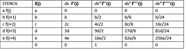
From the above Taylor table, equations extracted are
a + b + c + d + e = 0
b + 2c + 3d + 4e = 0
b/2 + 2c + 9d/2 + 16e/2 = 1
b/6 + 8c/6 + 27d/6 + 64e/6 = 0
b/24 + 16c/24 + 81d/24 + 256e/24 = 0
Now we have 5 equations and 5 variables which can be solved in MATLAB program, by which we can obtain a,b,c,d,e which can be solved in skewed right difference approximation.
% Calculation of skewed right difference coefficients
C = [1 1 1 1 1;0 1 2 3 4;0 1/2 4/2 9/2 16/2;0 1/6 8/6 27/6 64/6;0 1/24 16/24 81/24 256/24];
D = [0;0;1;0;0];
srd_coef = inv(C)*(D)
Taylor table for skewed left difference:

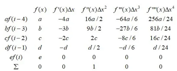
From the above Taylor table, equations extracted are
a + b + c + d + e = 0
- 4a - 3b - 2c - d = 0
16a/2 + 9b/2 + 2c + d/2 = 1
- 64a/6 - 27b/6 + 8c/6 - d/6 = 0
256a/24 + 81b/24 + 16c/24 + d/24 = 0
Now we have 5 equations and 5 variables which can be solved in MATLAB program, by which we can obtain a,b,c,d,e which can be solved in skewed right difference approximation.
Now doing the calculation of errors by central differencing methods using the analytical function in the formula for central differencing and their corresponding error difference with analytical derivative
%input variables
 x=pi/3
## f(x) = exp(x)*cos(x);

 dx = linspace(pi/20,pi/400,20)

 %analytical derivative
 analytical_deravative = -2*exp(x)*sin(x);

## Calculation of error for all differences
for i=1:length(dx)


%Calculating value and error by central difference methods
 central_diff(i) = (cd_coef(1)*f(x-(2*dx(i)))+cd_coef(2)*f(x-dx(i))+cd_coef(3)*f(x)+cd_coef(4)*f(x+dx(i))+cd_coef(5)*f(x+(2*dx(i))))/((dx(i))^2)
 err_cd(i) = abs(analytical_deravative-central_diff(i))
Now doing the calculation of errors by skewed right differencing methods using the analytical function in the formula for skewed right differencing and their corresponding error difference with analytical derivative
%Calculating value and error by skewed right difference methods
 right_sdiff(i) = (srd_coef(1)*f(x)+srd_coef(2)*f(x+dx(i))+srd_coef(3)*f(x+2*dx(i))+srd_coef(4)*f(x+3*dx(i))+srd_coef(5)*f(x+4*dx(i)))/(dx(i))^2
 err_sr(i) =abs(analytical_deravative-right_sdiff(i))
Now doing the calculation of errors by skewed left differencing methods using the analytical function in the formula for skewed left differencing and their corresponding error difference with analytical derivative
%Calculating value and error by skewed left difference methods
 left_sdiff(i)= (sld_coef(1)*f(x-4*dx(i))+sld_coef(2)*f(x-3*dx(i))+sld_coef(3)*f(x-2*dx(i))+sld_coef(4)*f(x-dx(i))+sld_coef(5)*f(x))/(dx(i))^2
 err_sl(i) = abs(analytical_deravative-left_sdiff(i))
Function program neede for running the f(x) function and save as f.m
function F = f(x)
 F= exp(x)*cos(x)
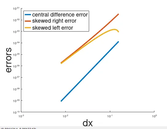
plotting the errors using the loglog plot for error central difference, error skewed right difference and the skewed left difference
%plotting of errors
figure(1)
hold on
loglog(dx,err_cd,'linewidth',3)
loglog(dx,err_sr,'linewidth',3)
loglog(dx,err_sl,'linewidth',3)
xlabel('dx','fontsize',32)
ylabel('errors','fontsize',32)
legend('central difference error','skewed right error','skewed left error','fontsize',18,'location','northwest')
The whole program.
clc;
clear all;
close all;

% Calculation of central difference coefficients
A = [1 1 1 1 1;-2 -1 0 1 2;2 1/2 0 1/2 2;-8/6 -1/6 0 1/6 8/6; 16/24 1/24 0 1/24 16/24];
B= [0;0;1;0;0];
cd_coef = inv(A)*(B)

% Calculation of skewed right difference coefficients
C = [1 1 1 1 1;0 1 2 3 4;0 1/2 4/2 9/2 16/2;0 1/6 8/6 27/6 64/6;0 1/24 16/24 81/24 256/24];
D = [0;0;1;0;0];
srd_coef = inv(C)*(D)

% Calculation of skewed left difference coefficients
E = [1 1 1 1 1;-4 -3 -2 -1 0;16/2 9/2 2 1/2 0;-64/6 -27/6 -8/6 -1/6 0;256/24 81/24 16/24 1/24 0];
F = [0;0;1;0;0];
sld_coef = inv(E)*(F)

 %input variables
 x=pi/3
## f(x) = exp(x)*cos(x);

 dx = linspace(pi/20,pi/400,20)

 %analytical derivative
 analytical_deravative = -2*exp(x)*sin(x);

## Calculation of error for all differences
for i=1:length(dx)


%Calculating value and error by central difference methods
 central_diff(i) = (cd_coef(1)*f(x-(2*dx(i)))+cd_coef(2)*f(x-dx(i))+cd_coef(3)*f(x)+cd_coef(4)*f(x+dx(i))+cd_coef(5)*f(x+(2*dx(i))))/((dx(i))^2)
 err_cd(i) = abs(analytical_deravative-central_diff(i))

 %Calculating value and error by skewed right difference methods
 right_sdiff(i) = (srd_coef(1)*f(x)+srd_coef(2)*f(x+dx(i))+srd_coef(3)*f(x+2*dx(i))+srd_coef(4)*f(x+3*dx(i))+srd_coef(5)*f(x+4*dx(i)))/(dx(i))^2
 err_sr(i) =abs(analytical_deravative-right_sdiff(i))

 %Calculating value and error by skewed left difference methods
 left_sdiff(i)= (sld_coef(1)*f(x-4*dx(i))+sld_coef(2)*f(x-3*dx(i))+sld_coef(3)*f(x-2*dx(i))+sld_coef(4)*f(x-dx(i))+sld_coef(5)*f(x))/(dx(i))^2
 err_sl(i) = abs(analytical_deravative-left_sdiff(i))


end

%plotting of errors
figure(1)
hold on
loglog(dx,err_cd,'linewidth',3)
loglog(dx,err_sr,'linewidth',3)
loglog(dx,err_sl,'linewidth',3)
xlabel('dx','fontsize',32)
ylabel('errors','fontsize',32)
legend('central difference error','skewed right error','skewed left error','fontsize',18,'location','northwest')
function
function F = f(x)
 F= exp(x)*cos(x)
Output plots