Week 7 - Simulation of a 1D Super-sonic nozzle flow simulation using Macormack Method
Aim:
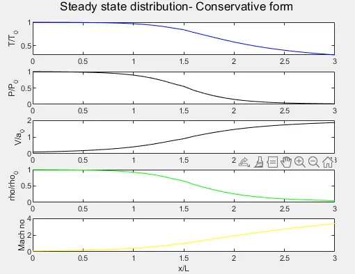
Derive derive both the conservation and non-conservation forms of the governing equations and sovle them using the MacCormack's technique. Also determine the steady-state temperature distribution for the flow-field variables and investigate the difference between the two forms of governing equations by comparing their solutions.
The main aim of this challenge is to implement all the CFD techniques which we have learned so far. In some
cases, more than one CFD technique will be used to solve the same flow problem. This is done to give you some comparison of
the strengths and weakness of one technique versus another and a feeling for the relative difficulty of setting up one technique
on the computer compared to another.
Macormack Method
In computational fluid dynamics, the MacCormack method is a widely used discretization scheme for the numerical solution of hyperbolic partial differential equations. This second-order finite difference method was introduced by Robert W. MacCormack in 1969. The MacCormack method is elegant and easy to understand and program
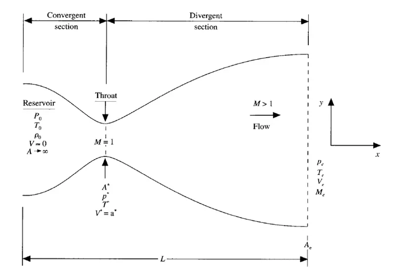
Representation of the flow by Macormack method
Predictor step
In computational fluid dynamics, the MacCormack method is a widely used discretization scheme for the numerical solution of hyperbolic partial differential equations.
Maccormacks method provides second order accuracy without the invlovement of second order derivative thus reducing the complexity of the calculation.It is a explicit method.
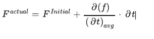
According to Maccormacks method the value of variable at grid point i,j at time t+dt is given as follows:
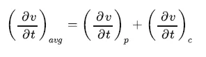
The average time derivative can be found as follows ,which is the half of sum of predicotor value and correcotr value .
So basically before that we need to set up equations for solving the predictor and corrector method.
Governing equations:
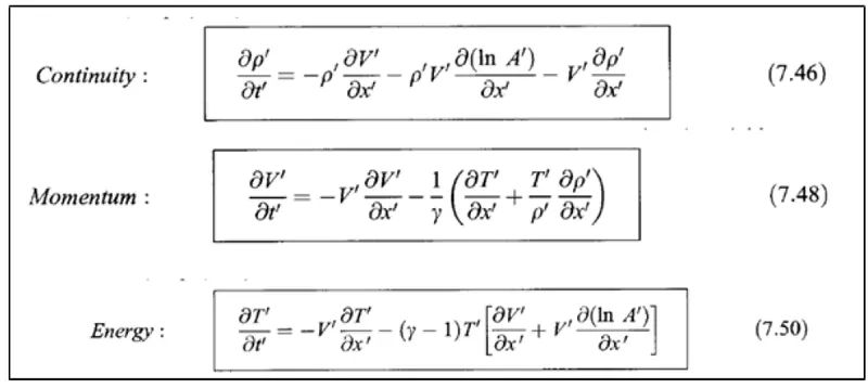
Non Conservative form
Conservative form
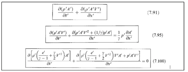
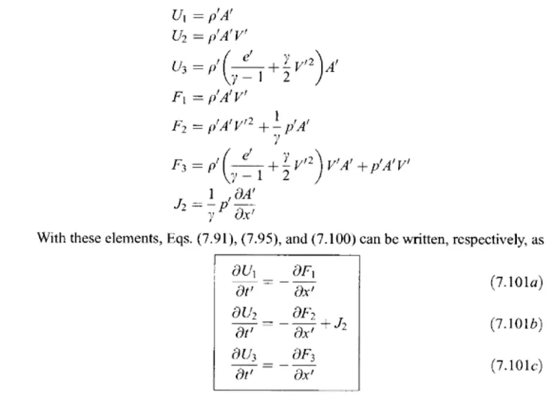
These are the equations we wish to solve numerically by using the MacCormacks technique.
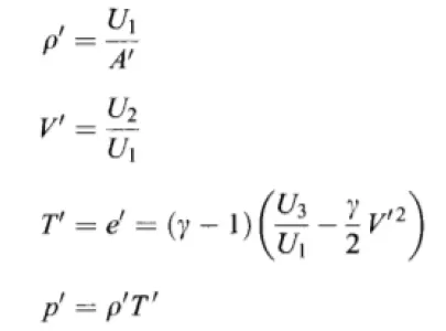
To obtain the primitve variables we must decode the elements U1,U2,U3 as follows.From the defination of U1,U2 and U3 given above we have
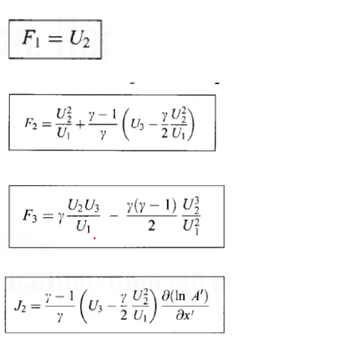
Expressing the flux and source term in form of solution vectors
Program non conservative
clear all
close all
clc

% inputs
n = 31
x = linspace(0,3,n);
dx = x(2)-x(1);

%Calculate initial profile
rho = 1-0.3146*x;
t = 1-0.2314*x; %t = temperature
v= (0.1+1.09*x).*t.^0.5;

%area
a = 1+2.2*(x-1.5).^2;

% Time steps
nt = 10;
dt = .001
gamma =1.4


% Outer time loop

for k = 1:nt

    % predictor method
    rho_old = rho;
    t_old = t;
    v_old = v ;
    % Continuity equation

    for j= 2:n-1

%         drho_dt_p = -rho(j)*(v(j+1)-v(j))/dx - rho(j)*v(j)*(log(a(j+1)-log(a(j)))/dx - v(j)*(rho(j+1) - rho(j))/dx
          dvdx = (v(j+1)-v(j))/dx;
          drhodx = (rho(j+1) - rho(j))/dx;
          dtdx = (t(j+1) - t(j))/dx;
          dlogadx = (log(a(j+1)-log(a(j))))/dx;

          % Continuity equation
          drhodt_p = -rho(j)* dvdx - rho(j)*v(j)* dlogadx -  v(j)* drhodx;

          % Momentum equation
          dvdt_p = -v(j)* dvdx -(1/gamma)*(dtdx + (t(j)/rho(j))*drhodx);

          % Energy equation
          dtdt_p = -v(j)* dtdx - (gamma- 1)* t(j)*(dvdx + (v(j)* dlogadx));

          %solution update
          rho(j) = rho(j) + drhodt_p*dt;
           v(j) = v(j)+ dvdt_p*dt;
           t(j) = t(j) + dtdt_p*dt;
    end

    % COrrector method

    for j= 2:n-1
%         drho_dt_c = -rho(j)*(v(j)-v(j-1))/dx - rho(j)*v(j)*(log(a(j)-log(a(j-1)))/dx - v(j)*(rho(j) - rho(j-1))/dx
          dvdx = (v(j)-v(j-1))/dx;
          drhodx = (rho(j) - rho(j-1))/dx;
          dtdx = (t(j) - t(j-1))/dx;
          dlogadx = (log(a(j)-log(a(j-1))))/dx;

          % Continuity equation
          drhodt_c = -rho(j)* dvdx - rho(j)*v(j)* dlogadx -  v(j)* drhodx ;

          % Momentum equation
          dvdt_c = -v(j)* dvdx -(1/gamma)*(dtdx + (t(j)/rho(j))*drhodx);

          % Energy equation
          dtdt_c = -v(j)* dtdx - (gamma- 1)* t(j)*(dvdx + (v(j)* dlogadx));

          %solution update
          rho(j) = rho(j) + drhodt_c*dt;
           v(j) = v(j)+ dvdt_c*dt;
           t(j) = t(j) + dtdt_c*dt;
    end

    % Compute the average time derivative

           drhodt = 0.5*(drhodt_p + drhodt_c);
           dvdt = 0.5*(dvdt_p + dvdt_c);
           dtdt = 0.5*(dtdt_p + dtdt_c);

     % final solution update

            for i= 2:n-1
                rho(j) = rho(j) + drhodt*dt
           v(j) = v(j)+ dvdt*dt
           t(j) = t(j) + dtdt*dt

            end

            % Apply the boundary condition
            % Inlet
            v(1) = 2 *v(2) -v(3)

            % Outlet
            v(n) = 2*v(n-1) - v(n-2)
            rho(n) = 2*rho(n-1) - rho(n-2)
            t(n) = 2*t(n-1) - t(n-2)

end

figure(1)
subplot(5,1,1)
plot(x,t,'b')
ylabel('T/T_{0}')
% subplot(5,1,2)
% plot(x,p,'k')
% ylabel('P/P_{0}')
subplot(5,1,2)
plot(x,v,'k')
ylabel('V/a_{0}')
subplot(5,1,3)
plot(x,rho,'g')
ylabel('rho/rho_{0}')
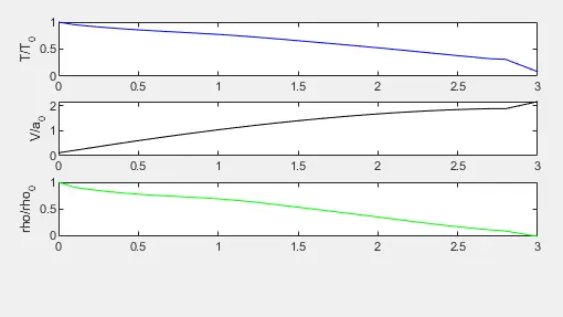
Output
Conservative program
clear all
close all
clc

% inputs
n = 31
x = linspace(0,3,n);
dx = x(2)-x(1);

%Calculate initial profile
% rho = 1-0.3146*x;
% t = 1-0.2314*x; %t = temperature
% v= (0.1+1.09*x).*t.^0.5;
%
%area
a = 1+2.2*(x-1.5).^2;
% Intial conditions
for i=1:length(x)
    if x(i)>= 0 && x(i)<= 0.5
        rho(i)=1;
        t(i)=1;
    elseif x(i)>=0.5 && x(i)<=1.5
        rho(i)=1-0.366*(x(i)-0.5);
        t(i)=1-0.167*(x(i)-0.5);
    elseif x(i)>=1.5 && x(i)<= 3.0
        rho(i)=0.634-0.3879*(x(i)-1.5);
        t(i)=0.833-0.3507*(x(i)-1.5);
    end
end

% Time steps
v=0.59./(rho.*a);
nt = 1400;
c = 0.5
dt=min(c.*dx./(sqrt(t)+v))
gamma =1.4

         u1 = rho.*a
          u2 = rho.*a.*v
          u3 = rho.*a.*((t./gamma -1)+ (gamma.* v.^2/2))
% Outer time loop

for k = 1:nt

    % predictor method
    u1_old = u1;
   u2_old = u2;
    u3_old = u3 ;


    for j= 2:n-1
         % Continuity equation
%        d(rho*a)_dt + d(rho*a*v)_dx = 0

%           f1 = rho*a*v
%           f2 = rho*a*v^2 + gamma^-1 *p*a
%           f3 = rho((e/(gamma -1 )+ ((gamma * v^2)/2))*v*a + rho*a*v
         f1 = u2
         f2 = ((u2.^2)./u1) + ((gamma-1)/gamma).*(u3 - ((gamma .* u2.^2)/2.*u1))
         f3 = ((gamma .* u2.*u3)./u1) - (gamma.*(gamma-1).*u2.^2/2.*u1.^2)
         j1(j) = (1/gamma)*rho(j)*t(j)*((a(j+1)-a(j))/dx);

%          predictor step


          % Continuity equation
          du1_dt_p(j) = (f1(j+1)-f1(j))/dx;

          % Momentum equation
          du2_dt_p(j) = (f2(j+1)-f2(j))/dx + j1(j);

          % Energy equation
         du3_dt_p(j) = (f3(j+1)-f3(j))/dx;

          %solution update
          u1(j) = u1_old(j) + du1_dt_p(j)*dt;
          u2(j) = u2_old(j) + du2_dt_p(j)*dt
          u3(j) = u3_old(j) + du3_dt_p(j)*dt
    end
        % The primitive variables are calculated from predictor solution vectors
    v=u2./u1;
    rho=u1./a;
    t=(gamma-1)*(u3./u1-(gamma/2).*v.^2);
    p = rho.*t;
    % Updating flux vectors from the predictor solution vectors
    f1=u2;
    f2=((u2.^2)./u1)+((gamma-1)/gamma)*(u3-((gamma*u2.^2)./(2*u1)));
    f3=(gamma*u2.*u3./u1)-(gamma*(gamma-1)/2)*(u2.^3./u1.^2);

    % COrrector method

    for j= 2:n-1
%       % Continuity equation
%        d(rho*a)_dt + d(rho*a*v)_dx = 0
%           u1 = rho*a
%           u2 = rho*a*v
%           u3 = rho*a((e/gamma -1)+ (gamma* v^2/2))
%           f1 = rho*a*v
%           f2 = rho*a*v^2 + gamma^-1 *p*a
%           f3 = rho((e/(gamma -1 )+ ((gamma * v^2)/2))*v*a + rho*a*v
         f1 = u2
         f2 = ((u2.^2)./u1) + ((gamma-1)/gamma)*(u3 - ((gamma.* u2.^2)/2.*u1))
         f3 = ((gamma.* u2.*u3)./u1) - (gamma.*(gamma-1).*u2.^2/2.*u1.^2)
%          f3 = ((gamma .* u2.*u3)./u1) - (gamma.*(gamma-1).*u2.^2/2.*u1^2)
         j2(j) = (1/gamma)*rho(j)*t(j)*((a(j)-a(j-1))/dx);

          % Continuity equation
         du1_dt_c(j) = (f1(j)-f1(j-1))/dx;

          % Momentum equation
         du2_dt_c(j) = (f2(j)-f2(j-1))/dx + j2(j)

          % Energy equation
         du3_dt_c(j) = (f3(j)-f3(j-1))/dx;

          %solution update
           u1(j) = u1_old(j) + du1_dt_c(j)*dt;
          u2(j) = u2_old(j) + du2_dt_c(j)*dt
          u3(j) = u3_old(j) + du3_dt_c(j)*dt
    end

    % Compute the average time derivative

           du1_dt = 0.5.*(du1_dt_p + du1_dt_c);
           du2_dt = 0.5.*(du2_dt_p + du2_dt_c);
           du3_dt = 0.5.*(du3_dt_p + du3_dt_c);

     % final solution update

            for m= 2:n-1
                u1(m) = u1(m) + du1_dt(m)*dt
                u2(m) = u2(m) + du2_dt(m)*dt
                u3(m) = u3(m) + du3_dt(m)*dt
           end

                rho = u1/a
                v = u2./u1
                t = (gamma-1).*(gamma-1).*((u3./u1) - ((gamma .* u2.^2)./2.*u1.^2))
                p = rho .* t

            % Apply the boundary condition
            % Inlet


end
figure(1)
subplot(2,1,1)
plot(x,t,'b')
ylabel('T/T_{0}')
subplot(2,1,2)
plot(x,p,'k')
ylabel('P/P_{0}')
subplot(2,1,3)
plot(x,v,'k')
ylabel('V/a_{0}')
subplot(2,1,4)
plot(x,rho,'g')
ylabel('rho/rho_{0}')
Output