Week 5.1 - Mid term project - Solving the steady and unsteady 2D heat conduction problem
Objective:
To solve the 2d heat conduction equation by using the point iterative techniques which includes the use of following the implicit methods
- Jacobi
- Gauss-seidel
- Successive over-relaxation
The boundary conditions are as follows
Top Boundary = 600 K
Bottom Boundary = 900 K
Left Boundary = 400 K
Right Boundary = 800 K
Error = 1e-4
Assume nx =ny = 10
Theory:
If the same is to be expanded for a three dimensional steady state
Now explaining the programs for steady state heat conduction Jacobi, Gauss seidal and sor methods
Jacobi steady state
First input the data like temps,nx,ny,,x,y dy,dx and k and then covergence loop and the nodal llops for condition then update old values
After that do the contour plot for x,y and t
 clear all;
 close all;
 clc;

 % inputs

 ny = 10
 nx = ny
 x = linspace(0,1,nx);
 y = linspace(0,1,ny);

 dx = x(2) - x(1)
 dy = y(2) - y(1)
 k= 2*(((dx^2)+(dy^2))/((dx^2 * dy^2)))


t = 300* ones(nx,ny);
t(1,:) = 600;
 t(nx,:) = 900;
 t(:,ny) = 800;
 t(:,1) = 400;
 t(1,1) = (400+600)/2;
 t(nx,ny) = (800+300)/2;
 t(1,nx) = (800+600)/2;
t(ny,1) = (900+400)/2;


 %Jacobi methods++
 tini = t;
 told = t;
 tol = 1e-4;

 %Calculation of solver using the Jacobi methods
 iterative_solver =1
 error = 9e9
 tol = 1e-4
 if iterative_solver == 1
   jacobi_iter = 1
    while(error > tol)
      for i = 2:nx-1
      for j = 2:ny-1
        t(i,j) = (1/k)*(((told(i-1,j) + (told(i+1,j)))/(dx^2)) + (told(i,j-1) + (told(i,j+1)))/(dy^2));
      end
      end

    error = max(max(abs(told - t)));
    told = t
    jacobi_iter = jacobi_iter + 1;
    end
  end
  contourf(x,y,t,'ShowText','on')
  set(gca,'ydir','reverse')
  sprintf( 'jacobi_iter = %d', jacobi_iter)
result
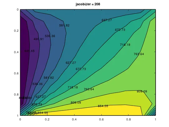
Jacobi steady implicit iteration number =208
Gauss seidal steady state
First input the data like temps,nx,ny,,x,y dy,dx and k and then covergence loop and the nodal llops for condition then update old values
After that do the contour plot for x,y and t
clear all;
 close all;
 clc;

 % inputs

 ny = 10
 nx = ny
 x = linspace(0,1,nx);
 y = linspace(0,1,ny);

 dx = x(2) - x(1)
 dy = y(2) - y(1)
 k= 2*(((dx^2)+(dy^2))/((dx^2 * dy^2)))


t = 300* ones(nx,ny);
t(1,:) = 600;
 t(nx,:) = 900;
 t(:,ny) = 800;
 t(:,1) = 400;
 t(1,1) = (400+600)/2;
 t(nx,ny) = (800+300)/2;
 t(1,nx) = (800+600)/2;
t(ny,1) = (900+400)/2;


 %Gaus seidal methods++
 tini = t;
 told = t;
 tol = 1e-4;

 %Calculation of solver using the Gauss seidal methods

 iterative_solver = 1
 error = 9e9
  tol = 1e-4;
if iterative_solver  ==1
       gs_iter = 1

  while(error > tol)
    for i = 2:nx-1
      for j = 2:ny-1
        t(i,j) = (1/k)*(((t(i-1,j) + (told(i+1,j)))/(dx^2)) + (t(i,j-1) + (told(i,j+1)))/(dy^2));
      end
     end
    error = max(max(abs(told - t)));
    told = t
    gs_iter = gs_iter + 1;
  end
end
   contourf(x,y,t,'ShowText','on')
  set(gca,'ydir','reverse')
  title(sprintf( 'gs_iter = %d', gs_iter))
Results
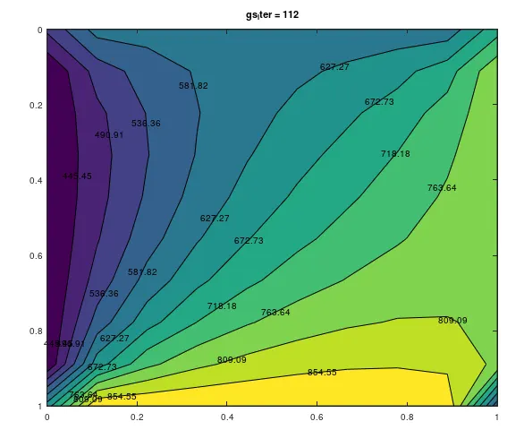
Gauss seidal iterations = 112
Succesive over relaxation
First input the data like temps,nx,ny,,x,y dy,dx and k and then covergence loop and the nodal llops for condition then update old values
After that do the contour plot for x,y and t
clear all;
 close all;
 clc;

 % inputs

 ny = 10
 nx =ny
 x = linspace(0,1,nx);
 y = linspace(0,1,ny);

 dx = x(2) - x(1)
 dy = y(2) - y(1)
 k= 2*(((dx^2)+(dy^2))/((dx^2 * dy^2)))
 omega = 1.5

t = 300* ones(nx,ny);
t(1,:) = 600;
 t(nx,:) = 900;
 t(:,ny) = 800;
 t(:,1) = 400;
 t(1,1) = (400+600)/2;
 t(nx,ny) = (800+300)/2;
 t(1,nx) = (800+600)/2;
t(ny,1) = (900+400)/2;


 %Sor methods++
 tini = t;
 told = t;
 tol = 1e-4;

 %Calculation of solver using the Successive over relaxation methods

 iterative_solver = 1
 error = 9e9
 tol = 1e-4;
 if iterative_solver ==1
       sor_iter =1
   while(error > tol)
    for i = 2:nx-1

      for j = 2:ny-1

        t(i,j) = ((1-omega)*told(i,j))+((omega)*((1/k)*(((t(i-1,j) + (told(i+1,j)))/(dx^2)) + (t(i,j-1) + (told(i,j+1)))/(dy^2))));
      end
    end

    error = max(max(abs(told - t)));
    told = t
  sor_iter = sor_iter + 1;
   end
end

  contourf(x,y,t,'ShowText','on')
  set(gca,'ydir','reverse')
  title(sprintf( 'sor_iter = %d', sor_iter))
Results
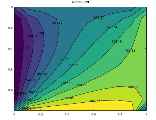
Sor no of iterations = 29
From the above three methods we can conclude that Sor has taken the least number of iteration(29) for the same nx and ny values and the next best is Gass seidal which took 112 iterations and Jacobi is the highest with 208 iterations
Unsteady/transient state
Jacobi unsteady
First input the data like temps,nx,ny,,x,y dy,dx,k1,k2,alpha and nt and then the time loop inside that the covergence loop and the nodal loops for condition then update old values
After that do the contour plot for x,y and t. for predefined values nt,nx,ny,dt and error terms
 clear all;
 close all;
 clc;

 % inputs

 ny = 10
 nx = ny
 x = linspace(0,1,nx);
 y = linspace(0,1,ny);
 dt=1e-3
 dx = x(2) - x(1)
 dy = y(2) - y(1)
 k= 2*(((dx^2)+(dy^2))/((dx^2 * dy^2)))
  alpha = 1.5

 k1 = (alpha*dt)/(dx^2);
  k2 = (alpha*dt)/(dy^2);

t = 300*ones(nx,ny);
t(1,:) = 600;
 t(nx,:) = 900;
 t(:,ny) = 800;
 t(:,1) = 400;
 t(1,1) = (400+600)/2;
 t(nx,ny) = (800+300)/2;
 t(1,nx) = (800+600)/2;
t(ny,1) = (900+400)/2;
nt = 100;


 %Assigning values of t

 tprev = t;
 told = t;
 tol = 1e-4;

 % Unsteady state using the Jacobi method
jacobi_iter =1
 for k=1:nt


    error = 9e9;
   while error > tol

     for i = 2:nx-1
       for j =2:ny-1

   term1 = (1+(2*k1)+(2*k2))^-1;
   term2 = k1*term1;
   term3 = k2*term1;
   H = (told(i-1,j) + told(i+1,j));
   V = (told(i,j-1) + told(i,j+1));
   t(i,j) = (tprev(i,j)*term1) + (H*term2) + (V*term3);
       end
     end

   error = max(max(abs(told - t)));
    told = t;
    jacobi_iter = jacobi_iter + 1;
  end
   tprev = t;
 end
figure(1)
   contourf(x,y,t,'ShowText','on')
  set(gca,'ydir','reverse')
  title(sprintf( 'jacobi_iter = %d', jacobi_iter))
Results
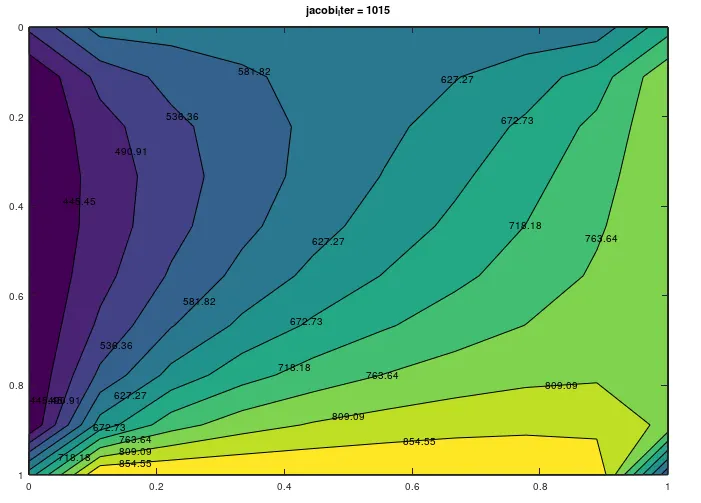
No of iterations for jacobi unsteady = 1015
2.Gauss -Seidal unsteady
First input the data like temps,nx,ny,,x,y dy,dx,k1,k2,alpha and nt and then the time loop inside that the covergence loop and the nodal loops for condition then update old values
After that do the contour plot for x,y and t. for predefined values nt,nx,ny,dt and error terms
 clear all;
 close all;
 clc;

 % inputs

 ny = 10
 nx =ny
 x = linspace(0,1,nx);
 y = linspace(0,1,ny);
  dt=1e-3
 dx = x(2) - x(1)
 dy = y(2) - y(1)
 k= 2*(((dx^2)+(dy^2))/((dx^2 * dy^2)))
   alpha = 1.5

 k1 = (alpha*dt)/(dx^2)
  k2 = (alpha*dt)/(dy^2)


t = 300*ones(nx,ny);
t(1,:) = 600;
 t(nx,:) = 900;
 t(:,ny) = 800;
 t(:,1) = 400;
 t(1,1) = (400+600)/2;
 t(nx,ny) = (800+300)/2;
 t(1,nx) = (800+600)/2;
t(ny,1) = (900+400)/2;
nt =100


 %Assigning values of t

 tprev = t;
 told = t;
 tol = 1e-4;

 % Unsteady state using the Gauss seidal method
gs_iter =1
 for k =1:nt

   error = 9e9;
   while error>tol
     for i = 2:nx-1
       for j =2:ny-1

   term1 = (1+(2*k1)+(2*k2))^-1;
   term2 = k1*term1;
   term3 = k2*term1;
   H = (t(i-1,j) + told(i+1,j));
   V = (t(i,j-1) + told(i,j+1));
   t(i,j) = (tprev(i,j)*term1) + (H*term2) + (V*term3);
      end
      end

   error = max(max(abs(told - t)));
   told = t;
    gs_iter = gs_iter + 1;
    end
    tprev = t
 end
 contourf(x,y,t,'ShowText','on')
  set(gca,'ydir','reverse')
  title(sprintf( 'gs_iter = %d', gs_iter))
Results
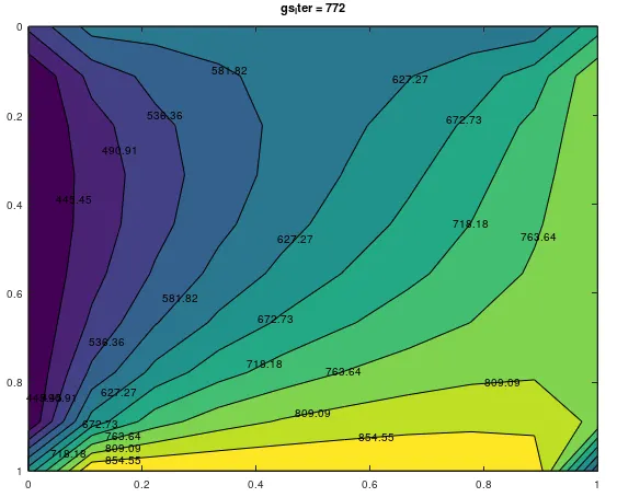
The number of iterations for gaauss seidal is 772
Successive over relaxation unsteady
First input the data like temps,nx,ny,,x,y dy,dx,k1,k2,alpha,omega and nt and then the time loop inside that the covergence loop and the nodal loops for condition then update old values
After that do the contour plot for x,y and t. for predefined values nt,nx,ny,dt and error terms
 clear all;
 close all;
 clc;

 % inputs

 ny = 10
 nx = ny
 x = linspace(0,1,nx);
 y = linspace(0,1,ny);
 dt=1e-3
 dx = x(2) - x(1)
 dy = y(2) - y(1)
 k= 2*(((dx^2)+(dy^2))/((dx^2 * dy^2)))
  alpha = 1.5
 omega =1.2

 k1 = (alpha*dt)/(dx^2)
  k2 = (alpha*dt)/(dy^2)

t = 300* ones(nx,ny);
t(1,:) = 600;
 t(nx,:) = 900;
 t(:,ny) = 800;
 t(:,1) = 400;
 t(1,1) = (400+600)/2;
 t(nx,ny) = (800+300)/2;
 t(1,nx) = (800+600)/2;
t(ny,1) = (900+400)/2;
nt = 100


 %Assigning values of t

 tprev = t;
 told = t;
 tol = 1e-4;

 % Unsteady state using the sor method
sor_iter =1
 for k = 1:nt
   error = 9e9;
   sor_iter = 1
   while error > tol
     for i = 2:nx-1
       for j =2:ny-1

   term1 = (1+(2*k1)+(2*k2))^-1;
   term2 = k1*term1;
   term3 = k2*term1;
   H = (t(i-1,j) + told(i+1,j));
   V = (t(i,j-1) + told(i,j+1));
   t(i,j) = ((1-omega)*told(i,j))+((omega)*((term1*tprev(i,j)) + (H*term2) + (V*term3)));
       end
     end

   error = max(max(abs(told - t)));
    told = t;
    sor_iter = sor_iter + 1;
   end
   tprev = t
 end
figure(1)
   contourf(x,y,t,'ShowText','on')
  set(gca,'ydir','reverse')
  title(sprintf( 'sor_iter = %d',sor_iter))
Results
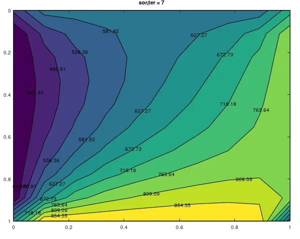
Sor iteration number = 7
So out of all of them implicit unsteady state sor iter has the lowest iteration number of 7 iterations
Explicit method
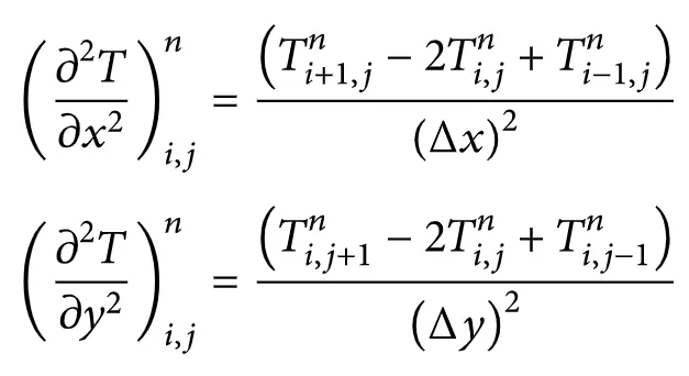
Explicit method is used in the numerical analysis for obtaining numerical approximathions to the solution of time dependent ordinary differential equations as in required in computer simulations.
This technique calculates the state of a system at a later time from the current time.


 clear all;
 close all;
 clc;

 % inputs

 ny = 10
 nx = ny
 x = linspace(0,1,nx);
 y = linspace(0,1,ny);
 dt=1e-3
 dx = x(2) - x(1)
 dy = y(2) - y(1)
## k= 2*(((dx^2)+(dy^2))/((dx^2 * dy^2)))
alpha = 1.5
 k1 = (alpha*dt)/(dx^2)
  k2 = (alpha*dt)/(dy^2)

t = 300*ones(nx,ny);
t(1,:) = 600;
 t(nx,:) = 900;
 t(:,ny) = 800;
 t(:,1) = 400;
 t(1,1) = (400+600)/2;
 t(nx,ny) = (800+300)/2;
 t(1,nx) = (800+600)/2;
t(ny,1) = (900+400)/2;
nt = 100


 %Assigning values of t

 tini = t;
 told = t;
 tol = 1e-4;

 % Unsteady state using the explicit method
explicit_iter =1
 for k=1:nt


     for i = 2:nx-1
       for j =2:ny-1

   term1 = told(i,j);
   term2 = k1*(told(i+1,j) - 2*told(i,j) +told(i-1,j));
   term3 = k2*(told(i,j+1) - 2*told(i,j) +told(i,j-1));
   t(i,j) = term1 + term2 + term3;
       end
     end

    told = t;
 end
figure(1)
   contourf(x,y,t,'ShowText','on')
  set(gca,'ydir','reverse')
  title(sprintf( 'explicit_iter = %d', nt))
Results
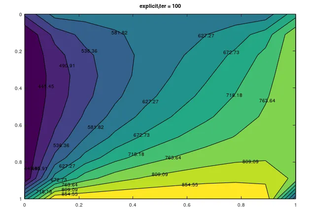
explicit method iteration number = nt which is equal to 100