week 2 : Image Filtering

Objective: Apply Prewitt and Laplacian filter on the image

Libraries used:

• Opencv
  • Open Source computer vision library.
  • cross-platform supported.
  • can perform through c, c++, and python.
• numpy
  • Mathematical library to work in the domain of Linear algebra, Fourier transform, and matrices.

Image Filtering in Image Processing is an important task, computing the local n at each position

Using filtering, we can enhance the image like Denoise, increase contrast and extract information like edges, lines ...

Detection of the edges and their orientations.

Theory :

• First Order Derivative Edge Detection. Generally, the first-order derivative operators are very sensitive to noise and produce thicker edges.
• Prewitt filter: The Prewitt operator is a discrete differentiation operator which functions similar to the Sobel operator, by computing the gradient for the image intensity function. Makes use of the maximum directional gradient. As compared to Sobel, the Prewitt masks are simpler to implement but are very sensitive to noise.
• Second Order Derivative Edge Detection. If there is a significant spatial change in the second derivative, an edge is detected. 2nd Order Derivative operators are more sophisticated methods towards automatized edge detection, however, are still very noise-sensitive.
• As differentiation amplifies noise, smoothing is suggested prior to applying the Laplacians. In that context, typical examples of 2nd order derivative edge detection are the Difference of Gaussian (DOG) and the Laplacian of Gaussian (LoG) (e.g.theMarr - Hildrethmethod).
• Firs order algorithms uses the simple pixel diferences for calculate the change gray intensity. On the other hand, second order algorithm employ the differneces among the central pixel and the both neighbor elements
• Prewitt and Laplacian are high pass filters that truncate the lower frequencies.
• Prewitt and Laplacian filters are used for Edge Detection.
• Both produce Binary Images.

Discrete First order Forward Difference along x and y:

`G_x ~~ f(x+1, y) - f(x, y)`

`G_y ~~ f(x, y+1) - f(x,y)`

Derivative mask of prewitt (1st order ) for 2D image:

• Veritcal filter (or) Mask:

`[[-1, 0, 1],[-1, 0, 1], [-1, 0, 1]]`

• Horizontal filter (or) Mask:

`[[-1, -1, -1],[0, 0, 0], [1,1, 1]]`

• In image processing, we consider pixel produce behaviour same with the local neighbourhood.
• So, Instead of taking derivative along the target pixel, we compare with neighbourhood pixels, to conclude whether an edge or not.

Derivative mak of Laplacian (2nd order):

`[[0, 1, 0],[1, -4, 1], [0, 1, 0]]` (or) `[[0, -1, 0],[-1, 4, -1], [0, -1, 0]]`

Second-order approximation of Taylor Series :

`(d^2)/(dx^2)f(x,y) = (d)/(dx)(df)/dx = (d)/(dx)[f(x+1, y) - f(x,y)] = (d)/(dx)f(x+1,y) - (d)/(dx)f(x,y)`

`= [f(x+1,y) - f(x,y)] - [f(x,y) - f(x-1,y)]`

`= f(x+1,y) - 2f(x,y) + f(x-1,y) = [[1],[-2],[1]]`

`(d^2)/(dy^2)f(x,y) = (d)/(dy)(df)/dy = (d)/(dy)[f(x, y+1) - f(x,y)] = (d)/(dy)f(x,y+1) - (d)/(dy)f(x,y)`

`= [f(x,y+1) - f(x,y)] - [f(x,y) - f(x,y-1)]`

`= f(x,y+1) - 2f(x,y) + f(x,y-1) = [1, -2, 1]`

Derivative mask of Laplacian captures both horizontal and vertical second-order derivative information.

An Edge Detector is called Optimal, if performs Good Detection and Good Localization.

Note :

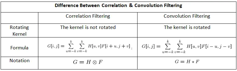
In ML and Image Processing, a convolution just defines the sliding of kernel over a feature map or image, flipping or no flipping normally not taken very seriously.

Thus in ML or image Processing someone moght talk of convolution and in actual sense it its cross-correlation (or) correlation upon close inspection.

In CNN, we call actully it a convolution, but it is actually cross-correlation.

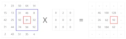
Fig : Filtering operation.

Functions Used:

• cv2.imread()
• cv2.resize()
• cv2.cvtColor()
• cv2.Laplacian()
• cv2.filter2D()
• cv2.addWeighted()
• cv2.convertScaleAbs()
• cv2.GaussianBlur()
• cv2.imshow()
• cv2.waitKey()
• cv2.destroyAllWindows()

Some Function Explanations :

• cv2.filter2D(source, dst, ddepth,kernel)
  • source - Image on which the filtering to perform.
  • dst - destination image size, shape and number of channels.
  • ddepth - depth of the image (data type), based on the filtering depth should be given, for gradients there may be a chance of float number. So np.float34 may provided.
  • kernel - Filter for convolution.

• cv2.Laplacian(source, dst, ddepth)
  • convolve laplacian derivative mask on the source image.

• cv2.convertScaleAbs(src, dst, ddepth)
  • convert float scale to the interger scale.

• cv2.addWeighted(src1, alpha, src2, beta, gamma)
  • This function used for blending operation.
  • alpha, (0 - 1) weighted importance for src1.
  • beta, (0 - 1) weighted importance for src2.
  • src1, src2 are source images.

• cv2.GaussianBlur(src, ksize, sigmaX, sigmaY, borderType)
  • src : Source/Input of n-dimensional array.
  • Ksize: Kernal is matrix of an (no. of rows)*(no. of columns) order .Its Size is given in the form of tuple (no. of rows, no. of columns). no. of rows and no. of columns should be odd .If ksize is given as (0 0), then ksize is computed from given sigma values i.e. sigmaX and sigmaY.
  • sigmaX : Standard deviation value of kernal along horizontal direction.
  • sigmaY : Standard deviation value of kernal along vertical direction.
  • border type : This specify boundaries of an image while kernel is applied on borders of an image.

    Possible values of borderType are :

    1. cv2.BORDER_CONSTANT : It adds a constant colored border. The value should be given as a keyword argument.
    2. cv2.BORDER_REPLICATE : The border will be mirror reflection of the border elements. Suppose, if image contains letters “abcdefg” then output will be “gfedcba|abcdefg|gfedcba“.
    3. cv2.BORDER_REPLICATE: It replicates the last element.
  • smoothens the image and noise also, do not remove. Consider only spatial distance, no photomrtric distance.

Code :

import cv2
import numpy as np

# inputs 

image = cv2.imread(r"C:UsersnarasOneDriveDesktopAytonomous Vehiclesskill lyncChallenge_2.png", 1)
image = cv2.resize(image, (700, 500))
gray_image = cv2.cvtColor(image, cv2.COLOR_BGR2GRAY)

# function definations

def perwitt_filter(image):
      
    vert_filter = np.array([[-1, 0, 1], [-1, 0, 1], [-1, 0, 1]])
    horz_filter = np.array([[-1, -1, -1], [0, 0, 0], [1, 1, 1]])
    
    vert_filtered = cv2.filter2D(image, -1, vert_filter)
    horz_filtered = cv2.filter2D(image, -1, horz_filter)
    
    abs_grad_x = cv2.convertScaleAbs(vert_filtered)
    abs_grad_y = cv2.convertScaleAbs(horz_filtered)

    final_image = cv2.addWeighted(abs_grad_x, 0.5, abs_grad_y, 0.5, 0)
    
    return final_image 

def laplacian_filter(image):

    filter1 = np.array([[0, 1, 0], [1, -4, 1], [0, 1, 0]])    
    filtered = cv2.filter2D(image, -1, filter1)    
    final_image = cv2.convertScaleAbs(filtered)
     
    return final_image 

def LoG(image):
    
    gauss_image = cv2.GaussianBlur(image, (5, 5), 3)
    return laplacian_filter(gauss_image)


# function calls

perwitt_image = perwitt_filter(gray_image)
laplacian_image = laplacian_filter(gray_image)
log_image = laplacian_filter(gray_image)

# Display the images

cv2.imshow("perwitt filtered image", perwitt_image)
cv2.imshow("laplacian filtered image", laplacian_image)
cv2.imshow("LOG filtered image", log_image)
cv2.imshow("laplacian and LOG", np.hstack((laplacian_image, log_image)))


cv2.waitKey(0)
cv2.destroyAllWindows()

Results :

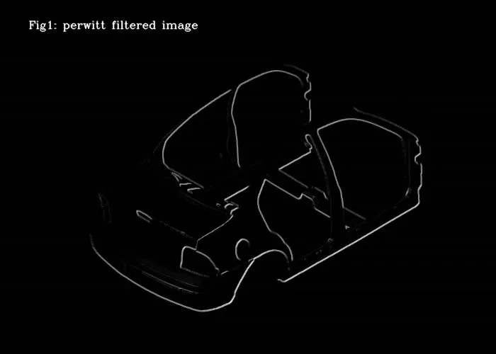
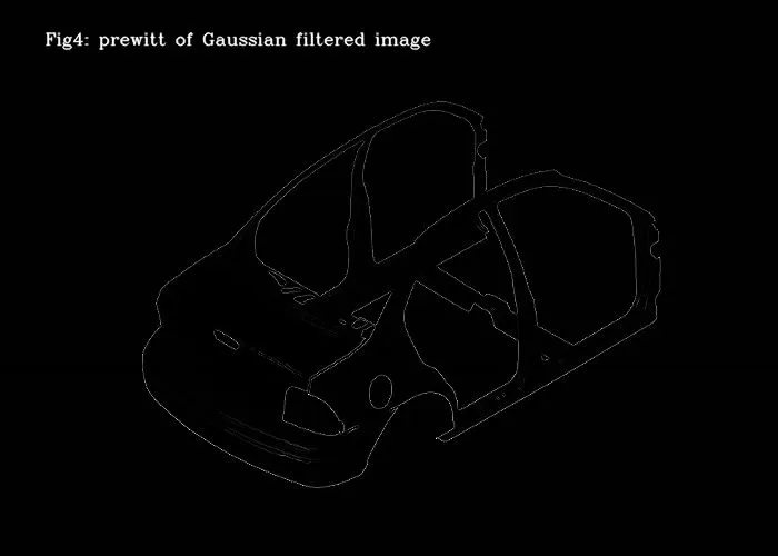
From Figure 1 & 3, Prewitt gives thicker edges due to very sensitive to the noise.

By appling the gaussian smoothing filter, the noise get dispersed more, using prewitt filter, got better edges.

In First Order Derivative masks, we consider threshold so higher chances for thicker edges.

But in Second Order Derivative masks, we say it is edges if the value is zero.

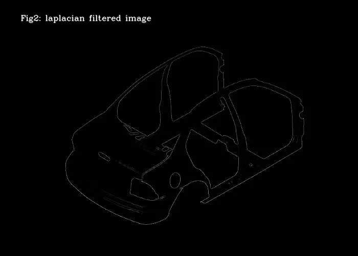
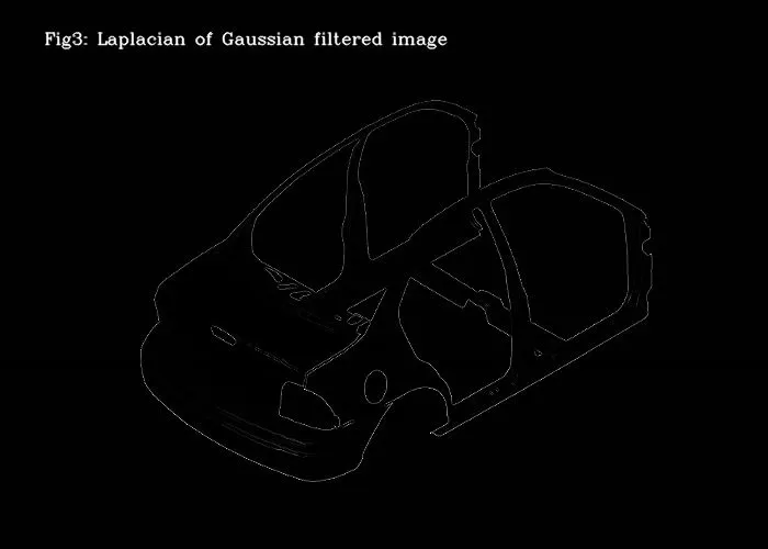
Laplacian filter provides good results than prewitt.

Applying LoG (Laplacian of Gaussian) filter, got more enhanced edges.

Conclusion :

1. Laplacian provides good defined edges than prewitt, even noise present.

2. After appying gaussian both providing good defined edges.

3. Prewitt is more simpler in implementation than Laplacian operation.