Week 2 - Flow over a Cylinder.
Aim: Simulation of Steady and unsteady flow over cylinder body.
Objective:
- Calculate the drag and lift coefficient over a cylinder by setting the Reynolds number to 10,100,1000,10000 & 100000 using a steady solver.
- Discuss the effect of Reynolds number on the coefficient of drag.
- Calculate the strouhal number for the unsteady case (Re = 100).
Introduction:
Fluid flow over solid bodies frequently occurs in practice, and it is responsible for numerous physical phenomena such as the drag force acting on automobiles, power lines, trees, and underwater pipelines, and the lift developed by bird or airplane wings; upward draft of rain, snow, hail, and dust particles in high winds
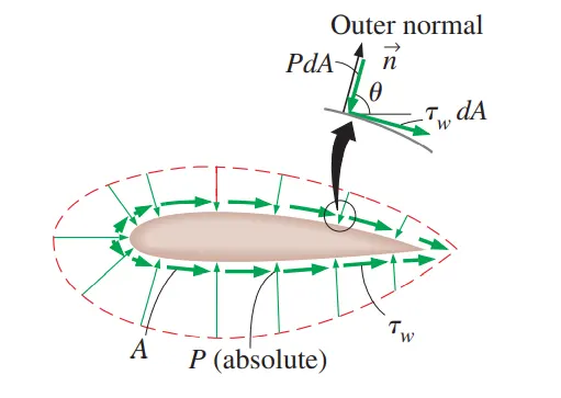
When a fluid moves over a solid body, it exerts pressure forces normal to the surface and shear forces parallel to the surface of the body.
The resultant pressure and shear forces component that acts in the flow direction is called the drag force (or just drag), and the component that acts normal to the flow direction is called the lift force (or just lift).
To calculate the drag and lift forces acting on any surface first step is to calculate the pressure and shear forces at a differential area dA on the surface which is PdA and twdA respectively.
In two-dimensional flow over an aerofoil, the drag force and lift force acting is given as,
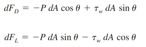
On the integration of the above equation over the entire surface we can get total drag and lift forces acting on the surface.
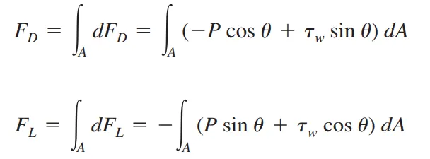
Using the same formula we can calculate the drag and lift force of any surface using which we can find a non-dimensional drag and lift coefficient of the body.
The coefficient of drag is the ratio of drag force to dynamic force, and the coefficient of lift is the ratio of lift force to dynamic force.
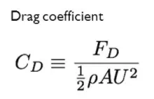
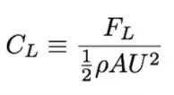
In this project, I will be simulating flow over cylinder body to capture flow separation, wake, stagnation point, vortex shedding, etc, and their effect on drag and lift coefficient, and effect of changing Reynolds number on drag and lift coefficient.
Geometry:
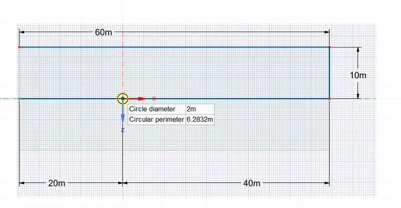
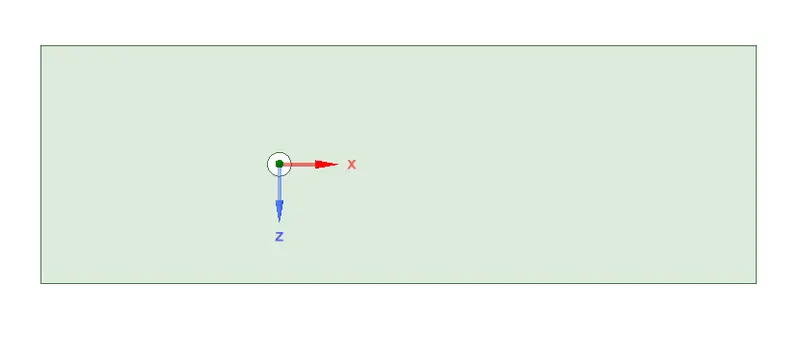
Geometry consists of the rectangular plate with a 2m hole which represents the cylinder body.
Meshing:
Edge meshing:
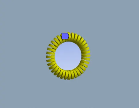
For sizing the mesh near a cylinder wall edge meshing is been applied (No of divisions = 36).
Inflation layer:
To accurately predict the boundary layer physics the inflation layer is added to the surface of the cylinder.
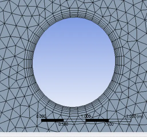
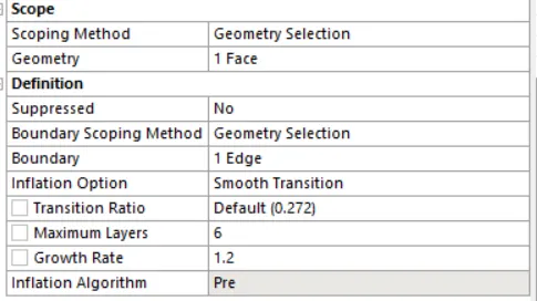
Final mesh:
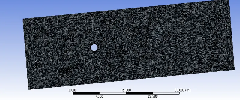
Setup:
Materials:
Material properties are been user-defined.
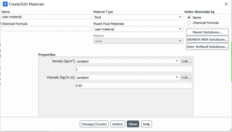
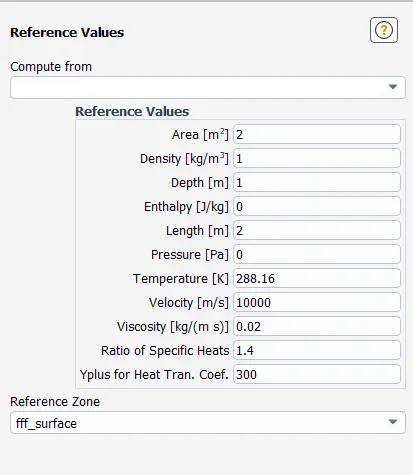
Reference values:
The area considered here is the frontal area seen by an observer standing at the inlet.
Solver:
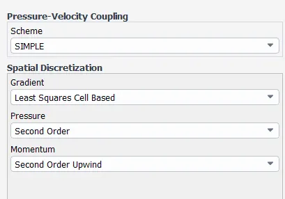
A simple solver is used because it is preferred for steady-state simulation.
Case1: Re = 10(Steady state)
Plots:
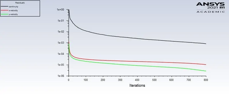
Residuals:
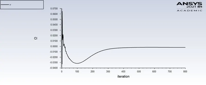
Lift coefficient:
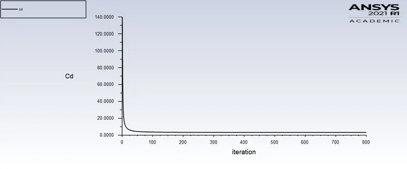
Drag coefficient:
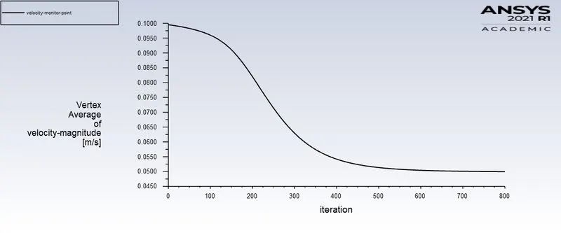
Velocity at monitor point:
Values:
Drag force and coefficient:

Lift force and coefficient:

Contours:
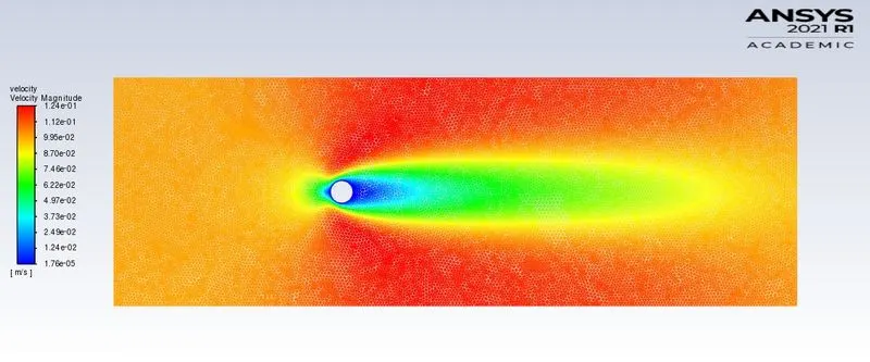
Velocity Contour:
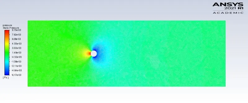
Pressure contour:
Case 2: Re = 100(Steady state)
Plots:
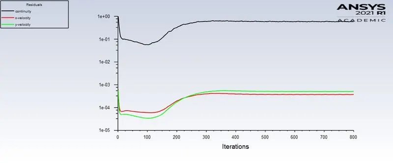
Residuals:
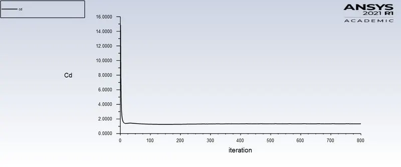
Drag coefficient:
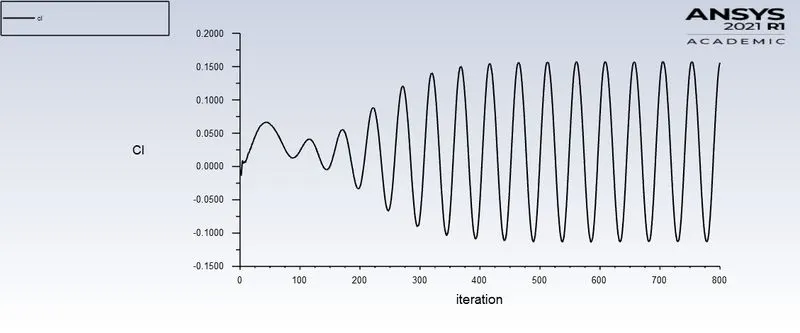
Lift coefficient:
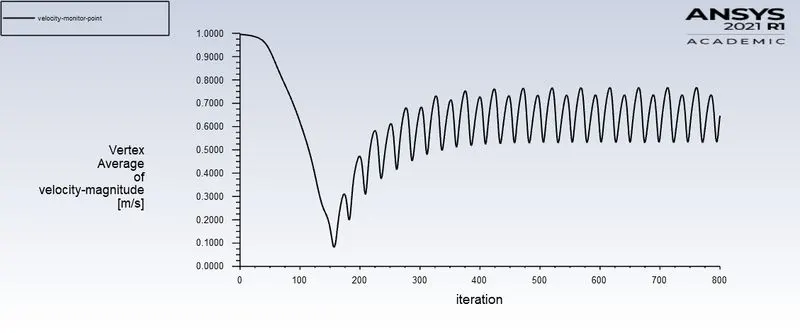
Velocity at monitor point:
Values:
Drag force and coefficient:

Lift force and coefficient:

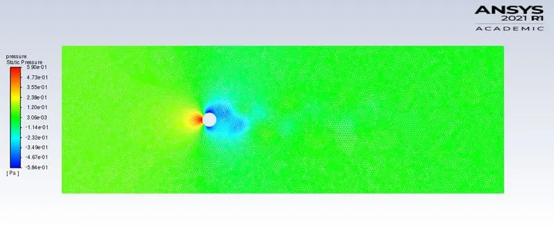
Contours:
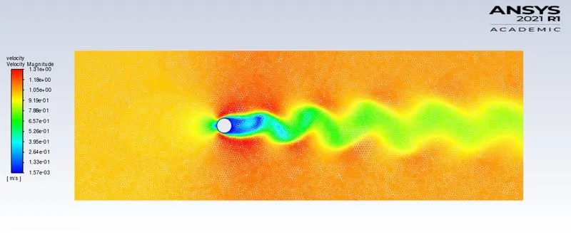
Velocity contour:
Pressure contour:
Case 3: Re = 1000
Plots:
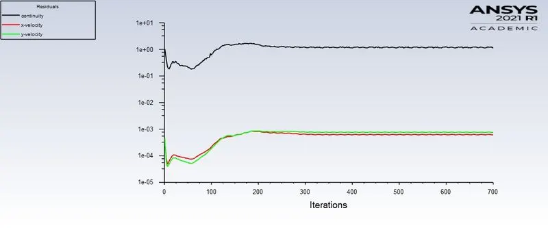
Residuals:
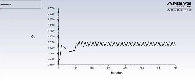
Drag coefficient:
Lift coefficient:
Velocity at monitor point:
Values:
Drag force and coefficient:

Lift force and coefficient:

Contours:
Velocity contour:
Pressure contour:
Vector:
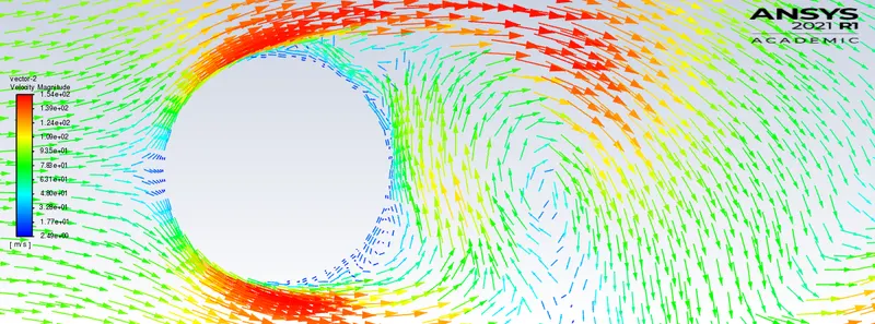
Velocity vector:
Case 4: Re = 10000(Steady state)
Plots:
Residuals:
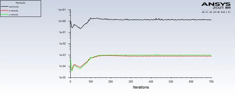
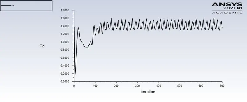
Drag coefficient:
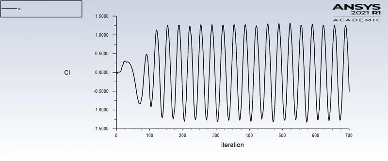
Lift coefficient
Values:
Drag force and coefficient:

Lift force and coefficient:

Contours:
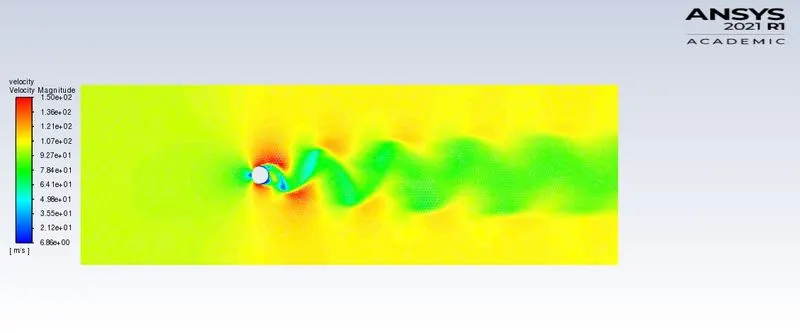
Velocity contour:
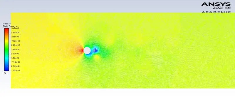
Pressure contour:
Vector:
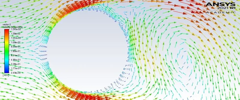
Velocity vector:
Case 5: Re = 100000(Steady state)
Plots:
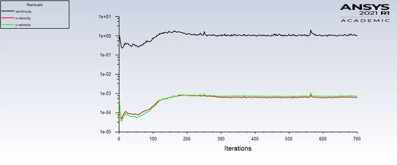
Residuals:
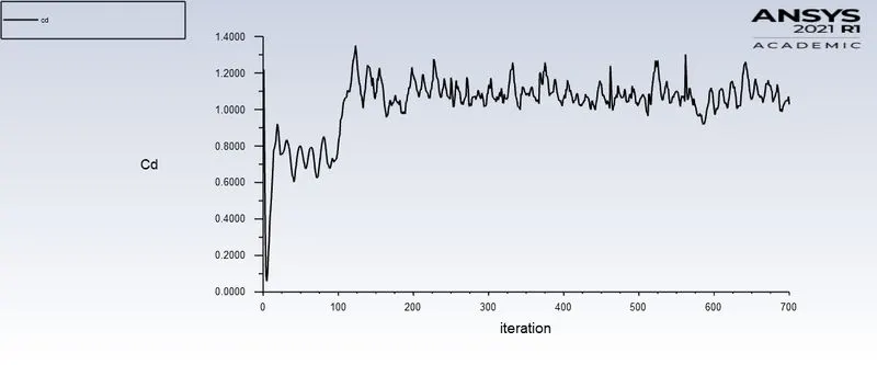
Drag co-efficient:
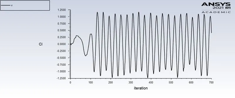
Lift coefficient:
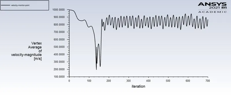
Velocity at monitor point:
Values:
Drag force and coefficient:

Lift force and co-efficient:

Contours:
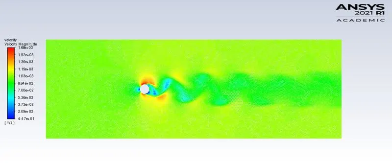
Velocity contour:
Vector:
Velocity vector:
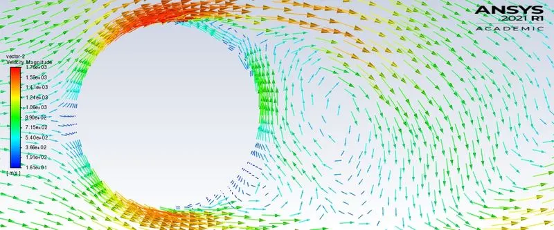
Case 6 : Re = 100 (Unsteady state)
Solver used: PISO
Plots :
Residuals:
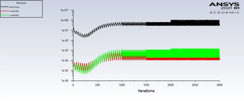
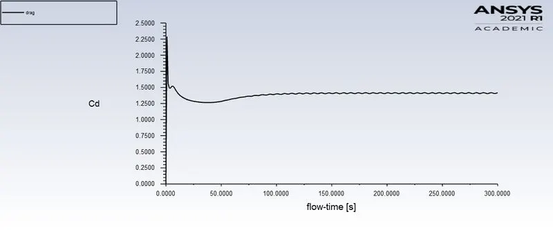
Drag coefficient:
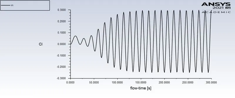
Lift coefficient:
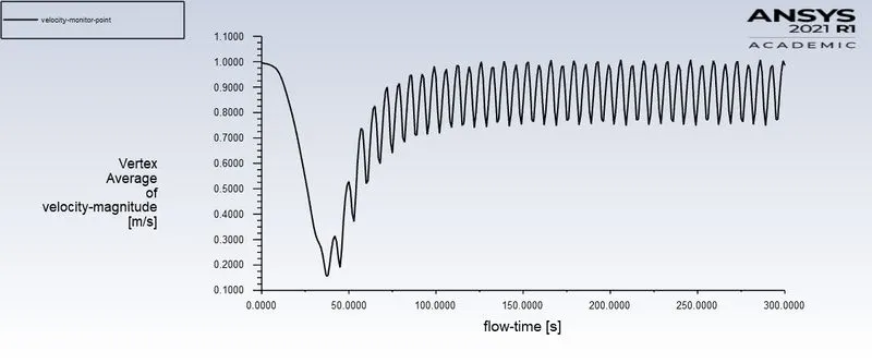
Velocity at monitor point:
Values:
Drag force and coefficient:

Lift force and coefficient:

Contours:
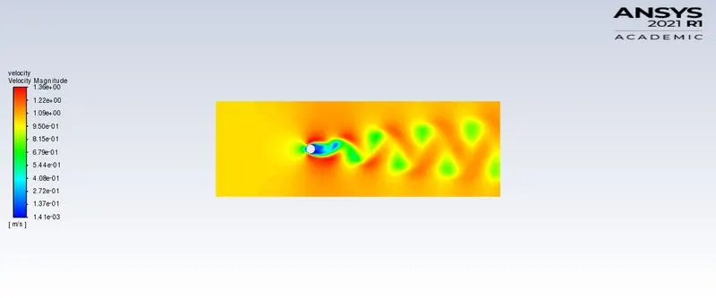
Velocity contours:
Vector:
Velocity vector:
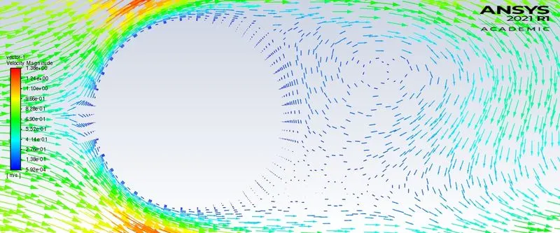
From vector plots for different Reynolds numbers, we can generally see the separation region near the wall of the cylinder.
Separation of boundary layers, in general, occurs when the velocity of the boundary layer “struggling” against an adverse pressure gradient becomes nearly zero, following the flow by reversing its direction.
- The separation point is defined as a location between forward and inverse flow where the wall shear stress is
zero. - The thickness of the boundary layer abruptly increases at the separation point, and the layer is forced off the
surface by the reversed flow near the wall. - Detached flow takes the form of vortical structures, which can be laminar or turbulent depending on the flow
regimes
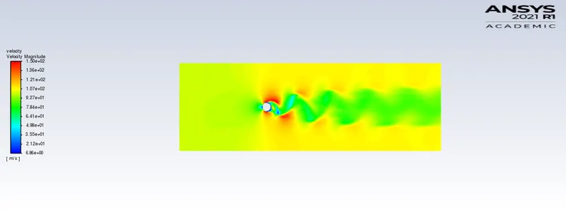
Boundary layer separation can, under a certain range of Reynolds numbers, generate a repeating pattern of vortices. This trail of vortices is called the Karman vortex street. which we get above Re = 100 for our simulation.
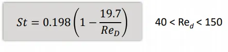
Vortex shedding in the Karman street locks into a self-sustained periodic pattern at a singular frequency (expressed in terms of non-dimensional Strouhal number) as
Forces induced on an object’s surface by periodic separation fluctuations have two distinct side effects as they:
‐ generate acoustic (sound) waves in a compressible fluid generating noise.
‐ Become culprits of resonant effects in the structure of the object when their frequency coincides with the natural frequency of the structure.
Strouhal number for unsteady state simulation:
St = fL/v
f = frequency of vortex shedding.
L = Characteristics length or diameter of cylinder in our case.
v = Velocity in m/s.
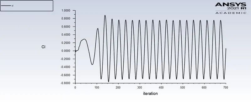
From the above lift plot number of vortex shedding can be said as 4 in between intervals (200 to 250).
f = 4/(250-200) = 0.08
St = f*L/v = 0.08*2/1 = 0.16
The strouhal number calculated from the Cl plot of unsteady flow is close to the value calculated using a formula which was been defined above for strouhal number in the range of (40< Re < 150) which is 0.1589.
Table for drag and lift(Steady state):
|
Reynolds number |
Drag coefficient |
Lift coefficient |
|
10(Steady state) |
3.336 |
-0.0018 |
|
100(Steady state) |
1.344 |
0.1557 |
|
100(Unsteady state) |
1.417 |
0.29 |
|
1000(Steady state) |
1.108 |
0.063 |
|
10000(Steady state) |
1.345 |
-0.5087 |
|
100000(Steady state) |
1.028 |
0.4046 |
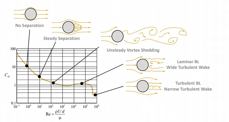
Variation of flow with Reynolds number(From reference):
Actual plot for different Reynolds numbers:
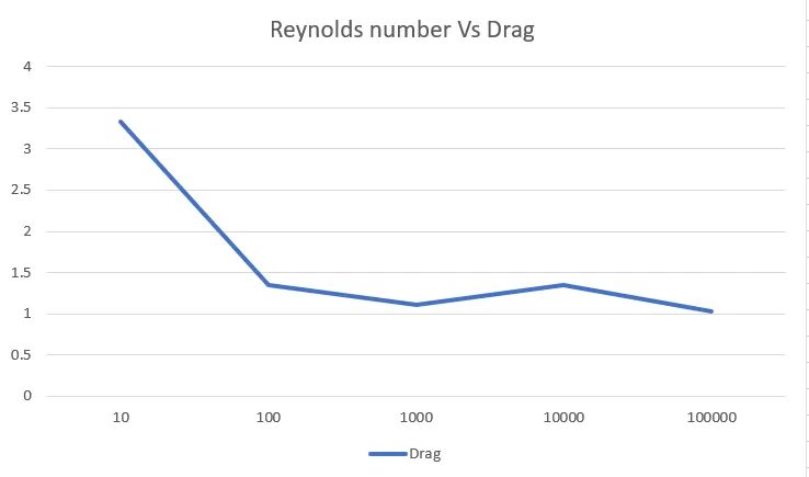
Inference:
- At low Reynolds numbers (Re < 1), the inertia effects are small relative to the viscous and pressure forces. In
In this flow regime, the drag coefficient varies inversely with the Reynolds number. - At moderate Reynolds numbers (1 < Re < 103), the flow begins to separate in a periodic fashion in the form of Karman vortices.
- At higher Reynolds numbers (103 < Re < 105), the flow becomes fully separated. An adverse pressure gradient
exists over the rear portion of the cylinder, resulting in the rapid growth of the laminar boundary and separation. - As the Reynolds number increases, the boundary layer becomes turbulent, delaying separation and resulting in
a sudden decrease in the drag coefficient. This effect is called the drag crisis. - The strouhal number for Reynolds number 100(unsteady case) is 0.16.