Week - 2 - Explicit and Implicit Analysis

Implicit and Explicit Methods

Explicit and implicit methods are two different approaches used in numerical analysis for calculating approximate numerical solutions to time-dependent ordinary and partial differential equations.

Implicit and explicit equations:

If we can represent the unknown variable in the equation in terms of known variables, ie if we can discriminate the variables then the equation is called an explicit equation.

eg: `y=lnx/x`, `x=e^(xy)`

Similarly, if we cannot discriminate the variables then the equation is called an implicit equation.

eg: `x^y=e^(xy)+x`

While implicit equations can be converted into explicit, it'll make the equation quite complex and more than one solution might be obtained.

In explicit method, dependent variables can be directly computed from the known quantities. But in case of implicit method, the unknown quantities to be calculated are expressed in terms of variables that are also unknown at the beginning. Therefore, iteration algorithms are necessary to achieve a numerical solution.

In CAE domain:

In the implicit method, the first solution is achieved from the initial values, followed by the evaluation of local element variables. If the convergence is not achieved, matrix coefficients should be recalculated with different time steps (known as iterations). In the implicit computational method, the stiffness matrix has to be inverted, which requires substantial computational power. Though the implicit solution is obtained using large time increments, the iterations and the calculation of the inverse stiffness matrix demand considerable memory and time. The implicit method is unconditionally stable. It is suitable for problems that tend to be highly linear, static, and quasi-static. Commercially available softwares for the application of implicit methods are ABAQUS, ANSYS, and NASTRAN.

In the explicit method, the unknown variables in the equation are expressed in terms of parameters calculated from the previous step. Therefore this method does not require iterations or inversion of the stiffness matrix which considerably reduces the computational power required. The disadvantage of the explicit method is its conditional stability. Although each increment of explicit time integration requires much less computational power, the time step has to be too small to provide stability to the explicit scheme. Thus the small timesteps demanded by the explicit scheme make it impractical for long-time processes. Commercially available softwares for the application of implicit methods are ls-dyna, radios, pamcrash, etc.

Thus the choice between implicit and explicit schemes depends on the type and size of the problem.

Salient features of implicit and explicit methods:

Explicit Scheme Implicit Scheme

• Suits problems having dynamic and inertial effects. Suits static and time-dependent problems.
• Do not require iterations. Requires iterations to solve equations.
• time step `Deltat`<`Delta t critical` Unconditionally stable. Solution will converge for any initial assumption of timestep
• Less accurate More accurate
• Consumes less time and memory Takes more time and memory
• Short timesteps is required for accurate results. larger timesteps can be implemented.
• Suitable for wave propagation, crash, drop, impact, blast etc. Good choice for problems with slow load rate (strain rate)
• Inverse of mass matrix [M] and damping matrix [C] is taken in CAE . Inverse of stiffness matrix [k] is taken, which is much simpler.

Aim:

Solve the given equation using both implicit and explicit methods and plot the graphs of the results.

A tolerance of 0.001 should be achieved in the Newton-Raphson iterations.

Eqtn : `F(u)=u^3+9u^2+4u`

Procedure:

A.Explicit Method

`F(u)=u^3+9u^2+4u`

`k(u)=(df)/(du)`=`3u^2+18u+4`

Step 1:

`u0=0`

`k(u0)=4,``DeltaF=1`

`Deltau1=(DeltaF)/(k(u0))=1/4`

`therefore u1=u0+Deltau1=0.25`

Step 2:

`u1=0.25, k(u1)=k(0.25)=8.6875`

`Deltau2=(DeltaF)/(k(u1)) = 1/8.6875 = 0.115`

`u2=u1+Deltau2= 0.25+0.115 =0.365`

Step 3;

`u2=0.365`

`k(u2)=k(0.365)=10.97`

`Deltau3=(DeltaF)/(k(u2))=1/10.97=0.091`

`u3=u2+Deltau3=0.365+0.091=0.456`

Substituting the final displacement in the force equation, we get the internal force developed in the material at the end of the displacement

as 3.79 N; which is not equal to the external force applied which means that the external and internal forces are not in equilibrium.

`Fext=DeltaF1+DeltaF2+DeltaF3=1+1+1=3`

`fi=(u3)^3+9(u3)^2+4u3=3.79`

Explicit Analysis Results Summary

Step i	`DeltaFi`	`Deltaui`	Ui	(Fext)i	(fint)i	R=fint-Fext
1	1	0.25	0.25	1	1.58	0.58
2	1	0.115	0.365	2	2.7	0.70
3	1	0.091	0.456	3	3.79	0.79

B.Implicit Method:

`F(u)=u^3+9u^2+4u`

`k(u)=(df)/(du)`=`3u^2+18u+4`

Step1:

`u0=0, k(u0)=4, DeltaF=1`

`Deltau1=(DeltaF)/(k(u0))=1/4` `therefore u1=u0+Deltau1=0.25`

Checking the residual

Fext= `Delta F`=1

fint=f(0.25) = 1.58

R(0)=fint-Fext=0.58

Since R(0) > 0.001 Newton-Raphson iteration is required to find the correction to u1

`deltau(1)=-[k(u1)(0)]^-1R(0)`

= `-[8.69]^-1*0.58=-0.0667`

updated value of `u1(1)=u1(0)+deltau(1)=0.25-0.0667=0.1835`

Checking the residual again:

fibnt=f(0.1835)=1.043

ie R(1)=1.043-1=0.043

since |R(1)| > 0.001, another iteration is required

Second iteration:

`deltau(2)= deltau(1)-[k(u1(1))]^-1*R(1)`

=-0.0665-[1/7.404]*0.043

=-0.0723

`u1(2)=u1(0)+deltau(2)`

=0.25+(-0.0723) = 0.1777

Checking the residual:

R(2)=fint(0.1777)-Fext=1.000607-1.000=0.000607

thus R(2)=0.000607 <0.001

therefore the final value of u1=u1(2)=0.1777

Step 2:

u1=0.1777, k(u1)=k(0.1777)=7.29333

`Delta F=1;Deltau2=(DeltaF)/(k(u1))=1/7.29333=0.137`

u2=u1+`Deltau2`=0.1777+0.137=0.3147

Checking the residual:

`Fext=DeltaF=2`

fint=f(0.3147)=2.1813

R(0)=2.1813-2.0=0.1813

since R(0) > 0.001, iterations are necessary

Calculating the correction to u2=u2(0)

`deltau2(1)=-[k(u2)(0)]^-1*R(0)`

=-[1/9.96]*0.1813

=0.0182

`u2(1)=u2(0)+deltau2(1)`

=0.3147+(-0.01819)

`u2(1)=0.2965`

Finding the residual:

Fext=2

fint=f(0.29651)=2.003372

R(1)=2.003372-2=0

since R(1)>0.001 one more iteration is necessary

Calculating the correction u2=u2(2)

`deltau2(2)=deltau2(1)-[k(u2(1))]^-1*R(1)`

=-0.01855125-[9.6]^-1*0.003372

`deltau2(2)=`=-0.01855125

`u2(2)=u2(0)+deltau(2)`

=0.3147+(-0.01855125)=0.29615

Residual, R(2) = fint(0.29615)-2.00 = 1.9999-2.0 = -0.0001

Since `|R(2)| = 0.0001 < 0.00`

Therefore final value of u2= u2(2) = 0.29615

Step 3:

`k(u2)=k(0.29615)=9.5938`

`DeltaF=1`

`Deltau3=(DeltaF)/(k(u2))=1/9.5938=0.1042`

`u3=u2+Deltau3`

`u3=0.29615+0.1042=0.4`

Checking the residual:

`R0=fi-Fext`

`=f(0.40035)-3=3.1080-3=0.1080`

R(0)=0.1080 > 0.001

Since R(0) >0.001, Iterations are necessary

Calculating the correction to u3=u3(0)

`deltau3(1) = -[k(u3(0))]^-1*R(0)`

=`[11.687]^-1*(0.1080)`

=-0.00924

`u3(1)=u3(0)+deltau3(1)=0.40035+(-0.00924)`

u3(1)=0.3911

checking the residual;

`R(1)=fi-Fext`

`f(0.39111)-3=3.00097-3=0.00097`

ie R(1)=0.00097<0.001

the final value of u3=u3(1)=0.3911

Implicit Analysis Results Summary

step (i)	`DeltaFi`	`ui`	`(Fex)i`	`(fInt)i`	R
1	1	0.1777	1	1.000607	0.000607
2	1	0.29615	2	1.9999	-0.0001
3	1	0.3911	3	3.00097	0.00097

Plot of Implicit Analysis Result Vs Actual Solution Plot of Explicit Analysis Result Vs Actual Solution

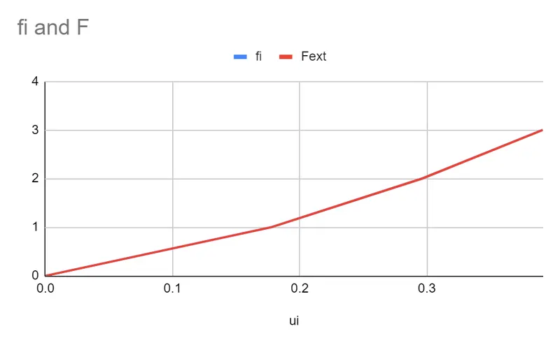
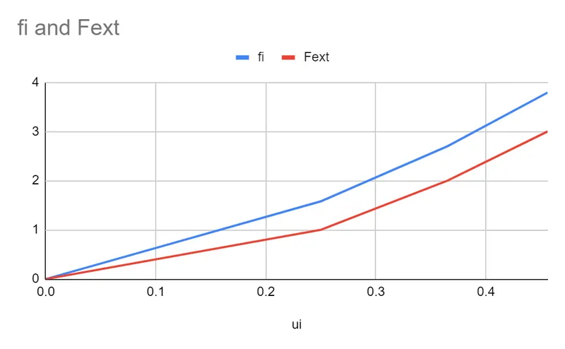
As seen from these graphs, the solution we got from implicit analysis matches the exact solution so perfectly that the curves are practically indistinguishable from each other, whereas the explicit solution graph lies, comparatively, much farther from the actual curve.