Week - 2 - Explicit and Implicit Analysis

AIM:

To solve the equation `F(u)=u^3+9u^2+4u` using explicit & implicit methods.

EXPLANATION:

Explicit:

An implicit solver solves the unknowns in the numerical equations by the inversion of the matrices that make up the model. Larger models have larger matrices. This is because of the large number of FE elements. Thus the analysis will take more time. When non-linearities are present in the model, the solution for the current time step is based on the solution from the previous time step. An implicit solver will produce solutions that are stable and allow for larger time increments.

Implicit:

An explicit analysis aims to solve for acceleration. The accelerations are solved for the nth time step, and then the velocity is solved for the n+1/2 step, and displacement at the n+1 step. The solutions are not always stable and much smaller time steps are required. The time step in an explicit analysis must be less than the time taken by a sound wave to travel across an element and is hence dependent on the mesh size and the material properties. This is known as the Courant time step.

`f(u) = u^3+9u^2+4u`

`k(u) = (df)/(df) = 3u^2+18u+4`

Explicit analysis:

Step 1

`u_0 = 0`

`k(u_0) = 0+0+4 = 4`

`Delta F =1`

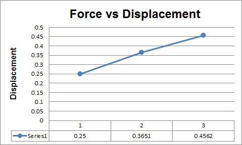
`Deltau_1 = (DeltaF)/(k(u_0) )=1/4 = 0.25`

`u_1=u_0+Deltau_1 = 0+0.25 = 0.25`

`f(u) = u^3+9u^2+4u = (0.25)^3+(9*0.0625)+(4*0.25)`

`f(u) = 1.5781`

Step 2

`k(u_1) = 0.1875+4.5+4 = 8.6875`

`Delta F =1`

`Deltau_2 = (DeltaF)/(k(u_1) )=1/8.6875 = 0.1151`

`u_2=u_1+Deltau_1 = 0.25+0.1151 = 0.3651`

`f(u) = u^3+9u^2+4u = (0.3651)^3+(9*(0.3651)^2)+(4*0.3651)`

`f(u) = 2.7078`

Step 3

`k(u_2) = 0.3998+6.5718+4 = 10.9716`

`Delta F =1`

`Deltau_3 = (DeltaF)/(k(u_2) )=1/10.9716 = 0.0911`

`u_3=u_2+Deltau_3 = 0.3651+0.0.0911 = 0.4562`

`f(u) = u^3+9u^2+4u = (0.4562)^3+(9*(0.4562)^2)+(4*0.4562)`

`f(u) = 3.7827`

Step i	`Delta F_i`	`Deltau_i`	`u_i`	`(F_(ext))_i`	`(f)_i`	`R = (f)_i-(F_(ext))_i`
1	1	0.25	0.25	1	1.5781	0.5781
2	1	0.1511	0.3651	2	2.7078	0.7078
3	1	0.0911	0.4562	3	3.7927	0.7927

Implicit analysis:

Step 1

`u_0 = 0`

`k(u_0) = 0+0+4 = 4`

`Delta F =1`

`Deltau_1 = (DeltaF)/(k(u_0) )=1/4 = 0.25`

`f(u) = u^3+9u^2+4u = (0.1834)^3+(9*0.1834)+(4*0.1834)`

`f(u) = 1.5781`

`R_1 = f-F = 1.5781-1 = 0.5781`

Since R1> 0.01 Newton-Raphson iterations are done

`x_1=x_0-f(x_0)/(f_1)(x_0)`

`Δu_1(1)=(R_1(1))/(k(1)u_1^(1)) = -0.066549`

`u_1(2) = u_1(1)+Δu_1(1)= 0.25-0.06654 =0.1834`

`F_1(2) = 1.04249`

`R_1(2) = 0.04249>0.01`

So Newton-Raphson method is applied

`Δu_1 (2) = (R_1(2))/(k(u_1^(2)))=0.07228`

`u_1(3) = u_1(2)+9(0.177^2)+4(0.177)=1.00075`

`R_1(3) = 0.000753 >0.01`

So Newton-Raphson method is applied

Thus,

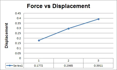
`u_1 =0.1772`

`f_1 = 1.0007`

`R_1=0.000753`

Step 2

`u_1 = 0.1772`

`k(u) = 3(0.1772^2)+18(0.1772)+4 = 7.29`

ΔF =1

`Δu_2= (ΔF)/(k(u)) = 0.137`

`u_2 = u_1+Δu_2 = 0.3148`

`f_2 = (0.177^3)+9(0.177^2)+4(0.177) = 2.182`

`R_2 = f_1 - F_1 = 0.1822`

As R2 > 0.01 Newton-Raphson method is applied

`Δu_2(1) = (R_2(1))/(k(u_2^(1))) = -0.018294`

`u_2(2) = u_2(1)+Δu_2(1)=0.3148-0.0182=0.2965`

`f_2(2) = 2.0037`

`R_2(2) = 0.00327<0.01`

So Newton-Rraphson method is not needed.

Thus,

`u_2 =0.2965`

`f_2 = 2.0032`

`R_2 = 0.003276`

Step 3

`u_2 = 0.2965`

`k(u) = 3(0.2965^2) +18(0.2965)+4 = 9.60073`

`ΔF=1`

`Δu_3 =(ΔF)/(k(u)) = 0.1046`

`u_3 = u_2+Δu_3 = 0.4006`

`F_3 = (0.296^3)+9(0.2965^2)+4(0.2965)`

`R_3 = f1-F1 = 0.111 > 0.01`

So Newton-Raphson method is applied

`Δu_3 (1) = (R_3(1))/(k(u_3^(1))) =-0.009493`

`u_3 (2) = u_3(1)+Δu_3(1)=0.3911`

`F_3(2) = 3.0008`

`R_3(2) = 0.00855<0.01`

Thus,

`u_3 = 0.3911`

`f_3 = 3.00855`

`R_3 = 0.00855`

Step i	`Delta F_i`	`Deltau_i`	`u_i`	`(F_(ext))_i`	`(f)_i`	`R = (f)_i-(F_(ext))_i`
1	1	0.07228	0.1772	1	1.0007	0.0007
2	1	-0.018294	0.2965	2	2.0032	0.0032
3	1	-0.009493	0.3911	3	3.00855	0.00855

Comparison of Explicit & Implicit methods:

CONCLUSION:

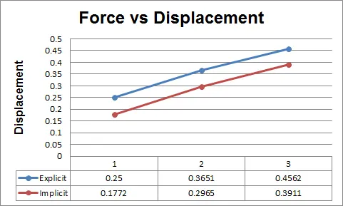
• Thus the given third-order polynomial equation under a tensile force is analytically solved both in the Implicit and Explicit methods. The results are plotted in the graph.
• From the graph, it is evident that implicit analysis is more accurate but time consuming and depends on element size and time steps whereas explicit analysis deviates slightly from the exact result and needs more iterations to obtain good results.