Week 2 Air standard Cycle

This project aims to build a code to solve the Otto cycle.

REQUIREMENT:

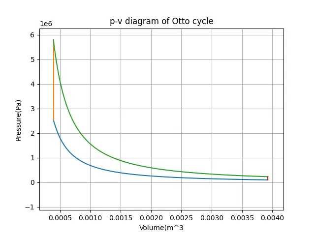
1. Your code should create a PV diagram

2. You should output the thermal efficiency of the engine.

THEORY:

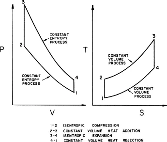
The Otto cycle is the theoretical cycle of interest when one is considering reciprocating SI engines. The four-stroke Otto cycle is made up of the following four internally reversible processes: 1–2, isentropic compression; 2–3, constant-volume heat addition; 3–4, isentropic expansion; and 4–1, constant-volume heat rejection.

The four-stroke Otto cycle is made up of the following four internally reversible processes:

1–2, isentropic compression

2–3, constant-volume heat addition

3–4, isentropic expansion

4–1, constant-volume heat rejection.

Basic overview:

Otto cycle is an air-standard cycle, the specific heat of air is 1.4

Initial conditions are assumed to be ambient values 350k and 101.325kPa respectively.

state variables and thermal efficiency are calculated using adiabatic process equations and ideal gas equation.

Since various values are generated, we need to create a different function that will keep storing the values of the generated variables which can later be used for plotting.

V array is set to null, after every iteration from the loop a new value is being stored using the append command and will be returning back after receiving desired values.

Python Code:

import math
import matplotlib.pyplot as plt

def engine_kinematics(bore,stroke,con_rod,cr,start_crank,end_crank):

	#engine geometric properties
	r = stroke/2
	n = con_rod/r 

	#Volume parameters
	v_swept = (math.pi/4)*pow(bore,2)*stroke
	v_clearance = v_swept/(cr-1)

	theta_startcrank = math.radians(start_crank)
	theta_endcrank = math.radians(end_crank)

	num_val = 100
	dtheta = (theta_endcrank- theta_startcrank)/(num_val-1)
	V = []
	for i in range(0,num_val):
		theta = theta_startcrank + i*dtheta
		term_1 = 0.5*(cr-1)
		term_2 = n+1 - math.cos(theta)
		term_3 = (pow(n,2) - pow(math.sin(theta),2))
		term_3 = pow(term_3,0.5)
		V.append((1+term_1*(term_2-term_3))*v_clearance)
	return V
#Input variables
gamma = 1.4
T3 = 2000
#state variable
#ambient conditions assumed
p1 = 101325
T1 = 350
#Engine geometry 
bore = 0.15
stroke = 0.2
con_rod = 0.8
cr =  10
#calculating swept volume and clerance volume 
v_swept = (math.pi/4)*pow(bore,2)*stroke
v_clearance = v_swept/(cr-1)
v1 = v_swept+v_clearance
v2 = v_clearance

#state variables at state point 2
#p2*v2*^gamma = p1*v1^gamma -------- Isentropic compression
p2 = p1*pow(cr,gamma)

#(p1*v1)/T1 = (p2*v2)/T2
#T2 = p2*v2*T1/(p1*v1)
T2 = p2*v2*T1/(p1*v1)
V_comp = engine_kinematics(bore,stroke,con_rod,cr,180,0)
C_const = p1*pow(v1,gamma)
P_comp = []
for v in V_comp:
	P_comp.append(C_const/pow(v,gamma))

#state variables at state point 3
v3 = v2  		#Isochronic process

#(p3*v3)/T3 = (p2*v2)/T2
#p3 = p2*T3/(T2)

p3 = p2*T3/(T2)
V_expp = engine_kinematics(bore,stroke,con_rod,cr,0,180)
C_const = p3*pow(v3,gamma)
P_expp = []
for v in V_expp:
	P_expp.append(C_const/pow(v,gamma))
#state variables at state point 4
v4 = v1			#Isocoric process
#p3*v3^gamma = p4*v4^gamma	#Isentropic expansion
p4 = p3*pow(v3,gamma)/ pow(v4,gamma)

#(p3*v3)/T3 = (p4*v4)/T4
#T4 = p4*v4*T3/(p3*v3)
T4 = p4*v4*T3/(p3*v3)

#plotting

plt.plot(V_comp,P_comp)
plt.plot([v2,v3],[p2,p3])
plt.plot(V_expp,P_expp)
plt.plot([v4,v1],[p4,p1])
plt.ylim([-5000000,8000000])
plt.xlim([0,0.005])
plt.xlabel('Volume(m^3')
plt.ylabel('Pressure(Pa)')
plt.title('p-v diagram of Otto cycle')
plt.grid()
plt.show()

Resulting plot: