Week 3 - Solving second order ODEs

OBJECTIVE:
To solve second order ODE using python

Converting second order ODE to two single order ODE

To stitch images to a GIF for a visual representation of second-order ODE functions

To write a program that solves the following ODE. This ODE represents the equation of motion of a simple pendulum with damping

PROCEDURE:

In Engineering, ODE is used to describe the transient behaviour of a system. A simple example is a pendulum

The way the pendulum moves depends on Newton's second law. When this law is written down, we get a second order Ordinary Differential Equation that describes "ball" w.r.t time period.

Similarly, there are hundreds of ODEs that describe key phenomena

We need to list the variables for the equation:

Governing equation:

`(d^2theta)/dt^2+b/m(d theta)/dt+ g/L sin theta =0`

Input values:

L=1 metre,

m=1 kg,

b=0.05.

g=9.81 m/s2.

import math
import matplotlib.pyplot as plt
import numpy as np
from scipy.integrate import odeint

#function
def model(T,t,b,l,g,m):
	T1 = T[0]
	T2 = T[1]
	dT1_dt = T2
	dT2_dt = -(b/m)*T2 -(g/l)*math.sin(T1)
	dTh_dt = [dT1_dt,dT2_dt]
	return dTh_dt
#inputs
b = 0.05 #damping co-efficient
l = 1
g = 9.81
m = 1

#initial conditions
T_x = [0,3]

#time points
t = np.linspace(0,20,150)
#solve ode
T = odeint(model,T_x,t,args=(b,l,g,m))

#plot
X = T[:,0]
ct = 1
for theta in X:
	x1 = 0
	y1 = 0
	x2 = l*math.sin(theta)
	y2 = -(l*math.cos(theta))
	file = 'test%05d.png' %ct
	plt.figure()
	plt.plot(t,T[:,0], '-',label = 'dispacement')
	plt.plot(t,T[:,1], '--',label = 'velocity')
	plt.ylabel('plot')
	plt.xlabel('time')
	plt.legend()
	plt.show()
	plt.plot([-1.5,1.5],[0,0],linewidth = 5)
	plt.plot([x1,x2],[y1,y2],linewidth = 4)
	plt.plot(x2,y2,'o',markersize = 12)
	plt.xlim([-1.5,1.5])
	plt.ylim([-1.5,1.5])
	plt.savefig(file)
	ct = ct+1

PLOTS:
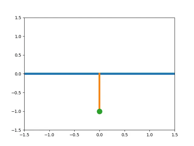
the following GIF is made from several images compiled together for time span of 20 seconds and we can see the damping effect of the pendulum.

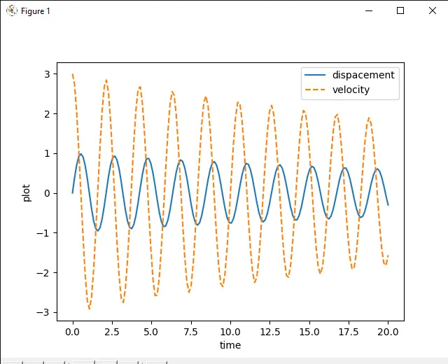
a follow-up plot can be plotted to check for the damping effect in terms of displacement and velocity, we can see that displacement was less gradual compared to the velocity.