Solving the equation using the Simulink block diagram and plotting the results.

Aim:

1. To plot the basic equation using the Simulink block.
2. To run and compare the suspension system

Objectives:

• The equation is given as `y(x)=(x-1)*(x-3)^2*(x-9)^2` is to be solved using the Simulink block diagram, and the result should be plotted for the given equation.
• The example in the help menu of Matlab of 'suspension system comparison' is to be run for the output and the results need to be explained.

Block diagram for the equation

The equation given is `y(x)=(x-1)*(x-3)^2*(x-9)^2`

The following is the block diagram for the above equation

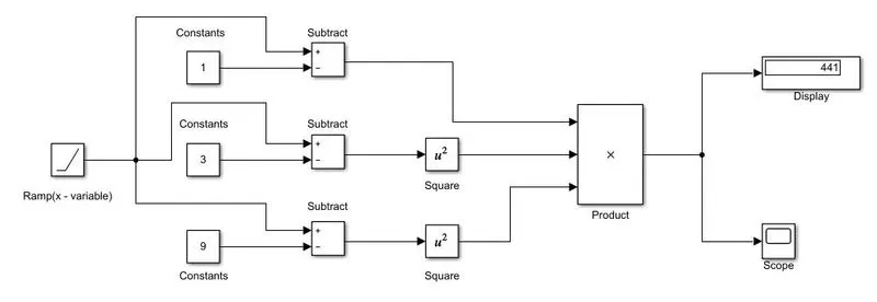
Explanation:

• As x is the variable the ramp function is used for representing the variable input to the diagram. The slope for the variable is taken 1.
• There are three constants that are represented in the equation, those are included as the constant values.
• Further, the operation is the subtraction, using the subtraction from the library. Two of the values need to be squared so will be adding the square term for the two values
• The final operation will be the product of all three values which will be displayed as a result and plotted in the scope.

Output:

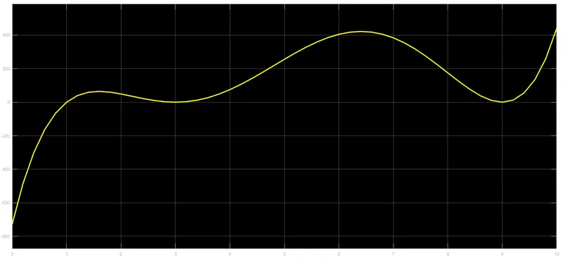
• As you can see in the output display the final answer is 441 i.e the last value after the complete function is been run. The above-mentioned plot is for the time duration of 10 seconds, so for the time of 10 seconds, the value of the function reached the maximum of 441.

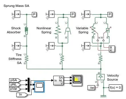
Block Diagram For the Suspension system

Questions

1. What is the objective of the simulation? What are the similarities and differences between the three systems of an understudy?

• The main objective of the simulation is to compare the three different types of suspension systems. The similarities between the three systems are they are connected to a common velocity source. All are provided with the constant value of tire stiffness.
• The only difference between the three systems is the main suspension mechanism. The first system is provided with the Shock Absorber, the second system is provided with the Nonlinear Spring, and the third system had a variable spring system.
• These three systems will behave differently for the same velocity input provided to them.

2. What are your observations from the results?

• The results for the above system are obtained as shown

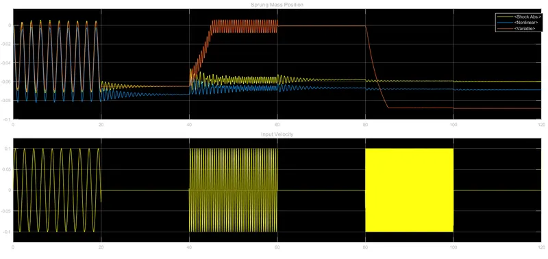
• As initially for the time of 0-20 sec, the oscillating frequency of 3 rad/sec all the three systems behave the same for the initial loading conditions.
• Later, the oscillations' frequency was increased from 3 rad/sec to 15 rad/sec for the time period of 40-60 sec. During this time period, the variable spring setup had the best damping of the oscillations while the liner and nonlinear spring damper had some vibration.
• For the next set of oscillations, the frequency was increased from 15 rad/sec to 75 rad/sec for the time duration of 80-100 sec the variable spring-mass system adjusts the mass in the setup to -0.09m for the minimum vibrations in the systems. while the linear and nonlinear setup has some amount of vibrations even after adjusting the masses in their system to -0.06m and -0.07m respectively.

3. How the oscillating velocity source is created?

The variable velocity system for the setup is made as shown below

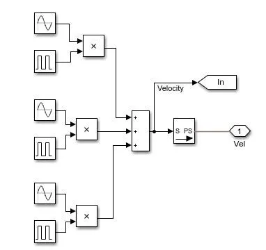
• The oscillating velocity source is created using three different sine wave functions, and three pulse generators.
• These two are then made into a product and finally added together to create the oscillating velocity.
• The three sine waves have the frequencies of 3 rad/sec, 15 rad/sec, and 75 rad/sec. The time for the pulse generator is 20 sec between each pulse.

Conclusion

From the above operations, we can conclude that the Simulink environment is suitable for solving various equations and other related problems. The example for the suspension system is clearly understood and the output is been clarified for better understanding.