Linear Convection for varying timesteps

AIM: To write a code for the linear convection for varying time step

OBJECTIVE:

Write a function that accepts the time step as an argument and solves the same problem. You will compare the effect of the time step on the numerical solution.

INPUTE

1. Number of nodes, n = 80

2. Time step , dt = 1e-4, 1e-3, 1e-2, and 1e-1

3. Simulation run time , t = 0.4 seconds.

4. Length L = 1m

5. The initial profile is a step function and it is 2m/s between x = 0.1 and 0.1 and 1m/s for the rest of the cycle.

6. Constant convective coefficient c = 1m/s

CODE

clc
clear all
close all

% Input for the linear convection problem
L = 1;
n = 81;
c = 1;
t = 0.4;
dt = [1e-4 1e-3 1e-2 0.0125 1e-1];
nt = t./dt;

x_start = 0.1;
x_stop = 0.3;

% calculation
x = linspace(0,L,n);
dx = x(2) - x(1);

for i = 1:length(x)
    a(i) = abs(x_start-x(i));
    b(i) = abs(x_stop-x(i));
end

n_start =find(a==min(a));
n_stop = find(b==min(b));

n_start_exact = find(x==0.4);
n_stop_exact = find(x==0.8);

%initial condition
u = ones(1,n);
u_exact = u;
u(n_start:n_stop) = 2;
u_exact(n_start_exact:n_stop_exact)=2;

u(1) = 1;
u_old = u;
u_initial = u;


for k = 1:length(dt)
    
    u = u_initial;
    u_old = u;
    
    cfl = c*dt(k)/dx;
    
    %time loop
    for m = 1:nt(k)
        %space loop
        for j = 2:length(x)
            u(j) = u_old(j)-cfl*(u_old(j)-u_old(j-1));
        end
        u_old = u;
    end
    
    figure(1)
    plot(x,u)
    axis([0 1 0 2])
hold on
xlabel('X-axis')
ylabel('velocity')
end

legend('1e-4dt','1e-3dt','1e-2dt','0.0125dt','1e-1dt')

EXPLANATION

• First, we are providing the various input for the linear convection problem

Length of the Domain(L),

No. of Nodes in an array(n),

Constant for the Velocity field(c),

Duration of the run time for the simulation(t),

No. of Time-steps(dt),

No. of time-marching steps(nt).

• Here, starting value is given by 'x_start' which is 0.1, and the ending value is given by x_stop which is given as 0.3.

• We're then creating equidistant mesh by setting up domain length from 0 to L and the no. of grid points for the value of the node provided in the challenge. The distance between two grids in the mesh is then given by dx.

• Now, we're defining another 'for' loop from 1 to length of 'x' to calculate the absolute values for the starting and ending positions of the square wave and storing it in variables 'a' and 'b' respectively.
• n_start takes the minimum value from the first array to calculate the starting node point & n_stop takes the minimum value from the second array to calculate the ending node point.
• Now, 'u' represents the boundary conditions for the given node which is starting from 'n_start_exact' and ending at 'n_stop_exact' and is given as 'u_exact'.
• Then we're creating a copy of the previous time step velocity field.
• After that, we're introducing a for loop in which using a range operator we're setting the length of timesteps from 1 to dt to calculate for all the values of timesteps.
• Then we're using the Courant number as a stability parameter. It is given as CFL = c*dt/dx where c is the flow velocity, dt is the representative time steps of the simulation and dx is the characteristic size of the mesh.
• In a CFD Simulation, the Courant number broadly indicates how much the information travels across a computational grid in a unit of time.
• Then we're setting up a time loop for all the timesteps and a space loop starting from 2 to the length of x.
• Finally, we're plotting the figure using plotting commands for their respective axes and providing the legends for various time steps.

OBSERVATION

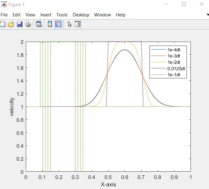
• The above figure shows the final velocity plot for the different time steps.
• AT dt = 1e-1, the solution is blowing up in ripples and oscillations hence proper velocity profile is not obtained because of the large value of time step causing a large value of CFL which makes the solution unstable.
• At de = 0.0125dt the peak value of the velocity profile is 2m/s as there is very little diffusion.
• For another remaining timestep, their final velocity profile is less than the initial value due to artificial diffusion which is caused due to an error term in the first-order approximation of the time and space derivative as it results in causing the velocity profile to lose its peak velocity gradient and sharpness.
• Change in time step size affects the numerical diffusion which brings instability based on the Courant Number (CFL)

CONCLUSION

Implicit Linear Convectionis are unconditionally stable as it also lacks a CFL condition. The happens as the implicit schemes use the entire domain to calculate each timestep and while solving an implicit linear system each timestep can result in adding time and cost. Also, the accuracy decreases as the timesteps increase.

Hence it is logical to use an explicit scheme with a lower timestep.