Simulation/Forward Kinematic of a 2R Robotic Arm using PYTHON

Simulation/Forward Kinematic of a 2R Robotic Arm

Objective:-

Development of a program in python to simulate the forward kinematics of a 2R Robotic Arm and to create an animation file of the plot.

Principle:-

Forward kinematics refers to the use of the kinematic equations of a robot to determine the position of the manipulator from specified values for the joint parameters. The kinematics equations of the robot are used in robotics and animation.

Solution Procedure:-

Robot kinematics refers to the analytical study of the motion of a robot manipulator, robotic arm is the most useful mechanical device which is used where accuracy and precision are needed. These things work similarly to the human arm and can be programmed as well. The traditional robotic arm will have n number of links, which are connected by joints with which links are rotated or translated. These links and joints form a Kinetic chain which has a Manipulator at the last link.

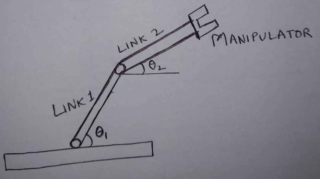
The above kinematics is made on Python

Steps Used-

Step 1 -: Calculating the position of Link 1

• Calculating the Start Point and the End Point for link 1

Start Point = (x0,y0) =(0,0)

End Point =(x1,y1) = (L1cos(theta1),L1sin(theta1)

Step 2 -: Calculating the position of Link 2

• Calculating the Start Point and the End Point for link 2

Start Point = (x1,y1) =(L1cos(theta1),L1sin(theta1))

End Point =(x2,y2) = (x1+L2cos(theta2),y1+L2sin(theta2))

Step 3 -: Calculating the Solution Set

[x0,y0],[x1,y1],[x2,y2]

Step 4 -:Plotting of a graph and its animation

We have used different values for each value of theta1 and theta2 for both links and stitch together to make an animation

_____________________________________________________________________________________________

CODE->

import math
import matplotlib.pyplot as plt

#Program for the forward kinematics of 2R robotic arm

#Inputs
l1=1
l2=0.5

n_theta= 10
theta_start =0
theta_end =math.pi/2

theta1=[]
theta2=[]

for i in range(0,n_theta):
	temp= theta_start + i*(theta_end -theta_start)/(n_theta-1)
	theta1.append(temp)
	theta2.append(temp)

#Base of the Robot
x0= 0
y0 = 0

ct=1
for t1 in theta1:
	for t2 in theta2:

		#link 1 ,link 2 connector
		x1 = l1*math.cos(t1)
		y1 = l1* math.sin(t1)
 
 		# Coordinates of the manipulator
		x2= x1+ l2*math.cos(t2)
		y2= y1+ l2*math.sin(t2)
		

		filename = 'test%05d.png' % ct
		ct=ct+1
		
		
		plt.figure()
		plt.plot([x0,x1],[y0,y1])
		plt.plot([x1,x2],[y1,y2])
		plt.xlim([0,2])
		plt.ylim([0,2])
		plt.savefig(filename)

Explanation of the code:-

• import math - to import the math class

• import matplotlib.pyplot as plt - to import the plotting library to plot graph

• #Program for the forward kinematics of 2R robotic arm - comments to make program user friendly

• #Inputs -comment

• l1=1 - initializing link 1 length as 1m

• l2=0.5 - initializing link 2length as 0.5 m

• n_theta= 10 -initializing with 10

• theta_start =0 - initializing the start of the theta with 0

• theta_end =math.pi/2 - initializing the end of the theta to 90 degree using math library

• theta1=[] - intializing an theta1 array to store the values

• theta2=[] - intializing an theta2array to store the values

• for i in range(0,n_theta): - for loop is used to execute the given statement in the range 0 to 9

• temp= theta_start + i*(theta_end -theta_start)/(n_theta-1) - initializing the temp value with 0 ,10,20,30,40,50,60,70,80,90 for different value to append in the theta1 and theta2 arrray

• theta1.append(temp) - append temp value in theta 1 array

• theta2.append(temp) - append temp value in theta 2array

• #Base of the Robot - comment

• x0= 0 - initializing link 1 coordinate as 0

• y0 = 0 - initializing link 1 coordinate as 0

• ct=1 - counter variable as 1

• for t1 in theta1: - for loop to execute given variables

• for t2 in theta2:- for loop to execute given variables

• #link 1 ,link 2 connector - comments

• x1 = l1*math.cos(t1) - initializing x1 coordinate

• y1 = l1* math.sin(t1) -initializing y1 coordinte

• # Coordinates of the manipulator - comment

• x2= x1+ l2*math.cos(t2) - initializing x2coordinate

• y2= y1+ l2*math.sin(t2) -initializing y2coordinte

• filename = 'test%05d.png' % ct - for arranging the png images in a orderly manner.Ex test00004,test00006.

• ct=ct+1 - incrementing the counter variable value by 1

• plt.figure() - to plot the graph a new figure window is created

• plt.plot([x0,x1],[y0,y1]) - to plot the graph

• plt.plot([x1,x2],[y1,y2]) - to plot the graph

• plt.xlim([0,2]) - to define limits to x axis

• plt.ylim([0,2]) to define limits to the y axis

• plt.savefig(filename) - to save the figure

Discussion:-

• The png file generated was stitched using the Imagemagick software to generate a gif
• Further converted to a video

Youtube link for the Simulation:-

https://youtu.be/q1cfUW-zudc