Mixing efficiency
AIM:- To study mixing efficiency of mixing Tee for different Momentum ratio.
Mixing Tee:- It is a device used in many mixing/diffusion process, and it also provide proper mixing of quantities to get desired result at output.
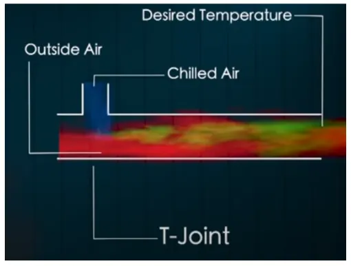
As shown in above figure, by adjusting chilled air velocity, we can get desired output.
Work flow of simulation:-
- Open Ansys workbench, double click/drag drop Fluid Flow (Fluent) analysis system to project schematic.

Here we see steps to follow to solve a CFD problem.
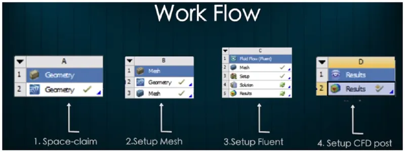
- Geometry: Spaceclaim, it is used for import the geometry and other CAD related functions like geometry clean-up etc.
- Mesh: used to generate Ansys Mesh and other mesh control option there, also assign name which helps during BCs steup.
- Setup: used to define physics of problem, like BCs, material, and type of solving method, iterations etc.
- Solution: where runtime results visualization done.
- Results: CFD-Post, where Post Processing of Results will be done.
Case 1:- Short Tee
- Geometry Cleanup:- Import short tee geometry into spaceclaim, spaceclaim gives various facility like CAD softwares, so we prepare geometry as per our simulation requirement.
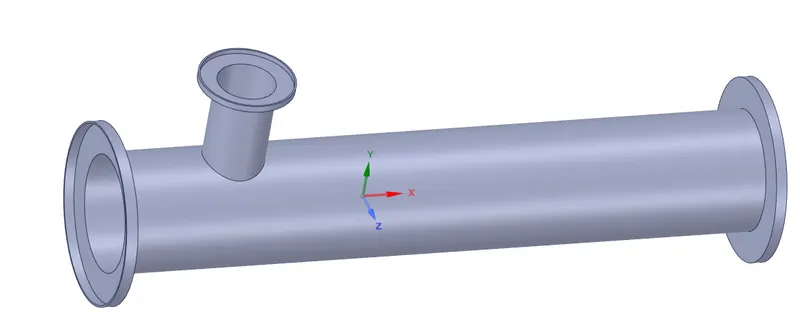
As per our simulation we are only interested in fluid flow analysis throught our short tee geometry, so we extract fluid volume from short tee geometry. Spaceclaim provide various option for extract the volume.
Goto Prepare -> Volume Extract -> Select edges
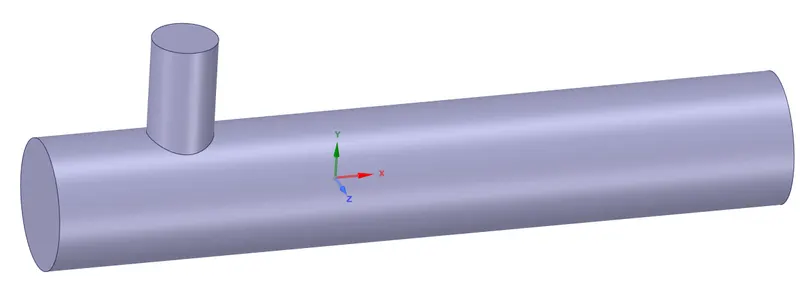
After extract flow volume, subpress for solid geometry so that it does not take part in mesh generation and futher simulation process.
b. Mesh Generation:-
In this step boundary naming also done. Boundary naming helps in for easy & correct visual of inlet/outlet and other geometry features so we can apply correct condition at correct place.
Mesh generation & element quality check is shown below-
we choose 1E-3 m element size.
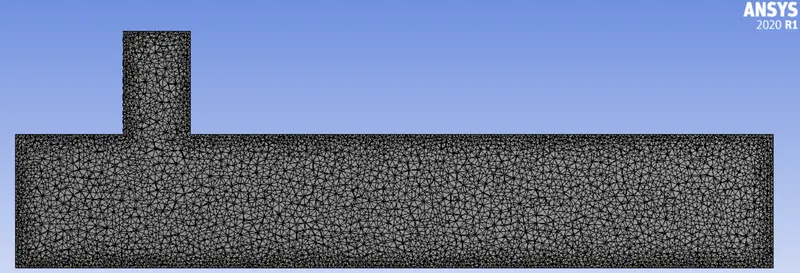
Goto Mesh -> Quality -> Mesh Metric -> Element Quality
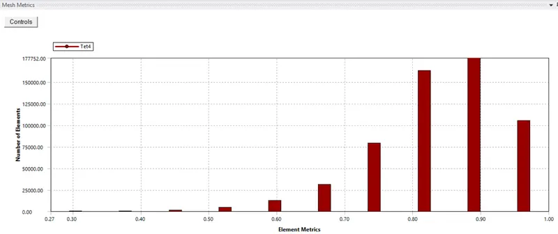
please check element quality should not be less than 5%.
c. Fluent Setup:-
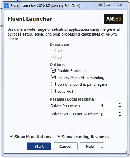
At Fluent launcher choose Double precision option & solver process.
Condition 1:-
Short Tee with a hot inlet velocity of 3 m/s & Momentum ratio of 2
| SETUP | K-epsilon | K-omega |
| Solver Type | Pressure Based | Pressure Based |
| Velocity Formulation | Absolute | Absolute |
| Time | Steady | Steady |
| Viscous Model | Realizable k-epsilon with standard wall function | k-omega SST model |
| Material | Air | Air |
| Cell Zones | ||
| Volume_Volume | Fluid type- Air | Fluid type- Air |
| Inlet x (velocity inlet) | Inlet x (velocity inlet) | |
| Velocity Magnitude= 3 m/s | Velocity Magnitude= 3 m/s | |
| Temp.= 36 degree C | Temp.= 36 degree C | |
| Boundaries | Inlet y (velocity inlet) | Inlet y (velocity inlet) |
| Velocity Magnitude= 6 m/s | Velocity Magnitude= 6 m/s | |
| Temp.= 19 degree C | Temp.= 19 degree C | |
| Outlet (pressure outlet) | Outlet (pressure outlet) | |
| Gauge Pressure= 0 pas. | Gauge Pressure= 0 pas. | |
| Walls= Stationary walls | Walls= Stationary walls |
After placing all input condition solution is initialize by Hybrid Initialization.
d. Results:-
For k-epsilon model For k-omega model
Residuals plot:-
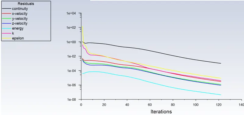
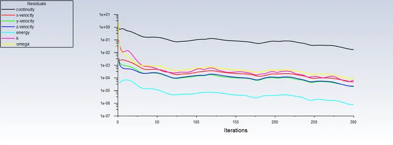
Approx. 122 iterations taken to converge solution. Approx. 250 iterations taken to converge solution.
Average weighted area Plot for Temp.:-
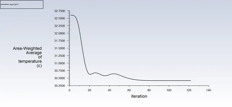
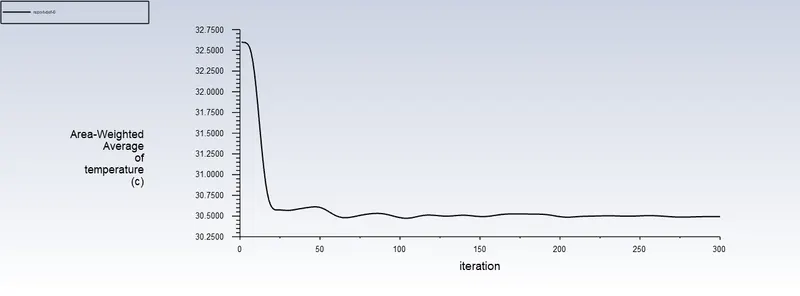
From the above snap outlet temp. of mixture is 30.4 degree C. From the above snap outlet temp. of mixture is 30.5 degree C
Standard deviation plot:-
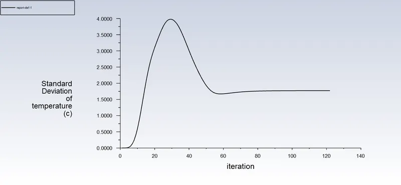
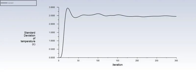
From the above snap standard deviation is 1.77 From the above snap standard deviation is 2.45
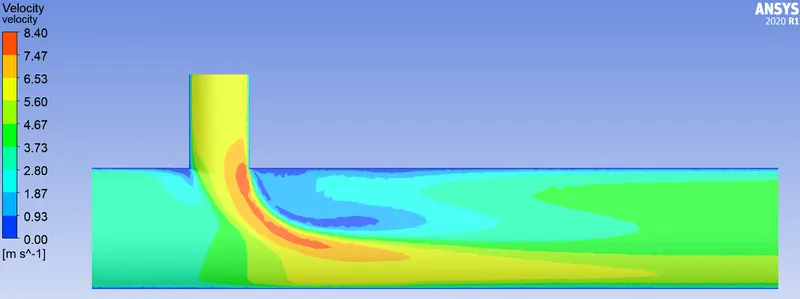
Contour plots:-
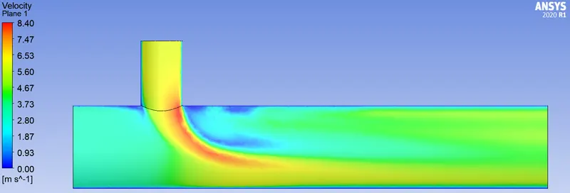
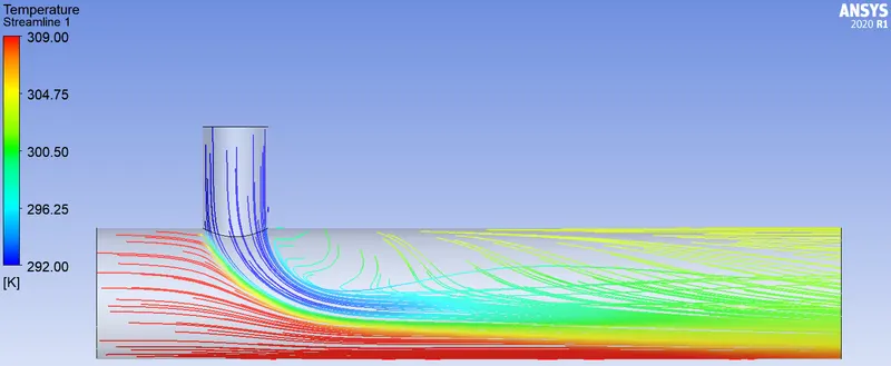
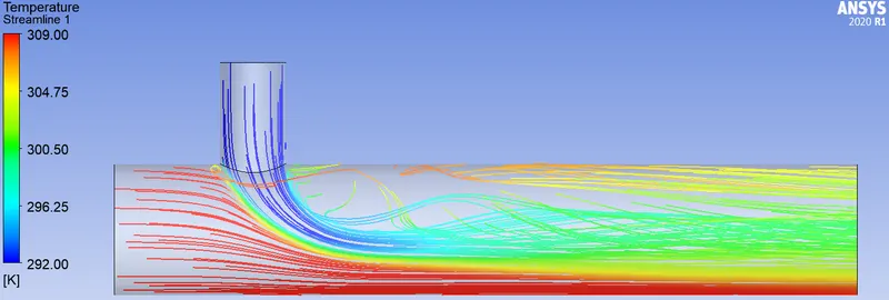
1) For Temp. distribution
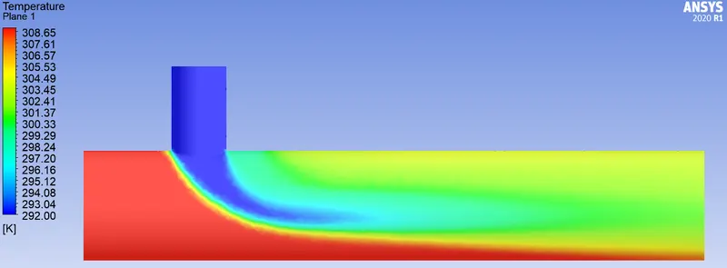
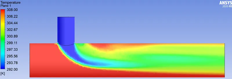
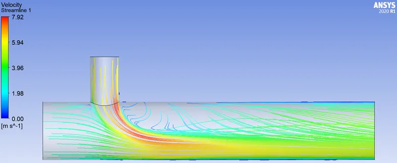
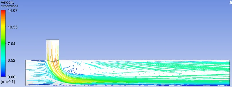
2) For Velocity. distribution
Line plots:-
1) For Temp. distribution
2) For Velocity. distribution
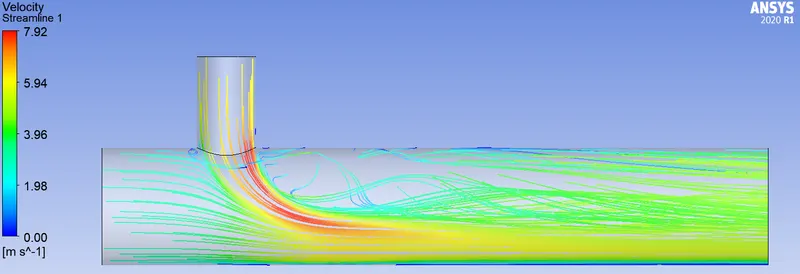
Summary:- Short Tee with MR=2
| K-epsilon | K-omega | |
| Cell count | 573264 | 573264 |
| Avg. Outlet Temp. | 30.4 degree C | 30.5 degree C |
| No. of Iterations | approx. 122 | approx. 250 |
| Standard deviation | 1.77 | 2.45 |
Short Tee with a hot inlet velocity of 3 m/s & Momentum ratio of 4
| SETUP | K-epsilon | K-omega |
| Solver Type | Pressure Based | Pressure Based |
| Velocity Formulation | Absolute | Absolute |
| Time | Steady | Steady |
| Viscous Model | Realizable k-epsilon with standard wall function | k-omega SST model |
| Material | Air | Air |
| Cell Zones | ||
| Volume_Volume | Fluid type- Air | Fluid type- Air |
| Inlet x (velocity inlet) | Inlet x (velocity inlet) | |
| Velocity Magnitude= 3 m/s | Velocity Magnitude= 3 m/s | |
| Temp.= 36 degree C | Temp.= 36 degree C | |
| Boundaries | Inlet y (velocity inlet) | Inlet y (velocity inlet) |
| Velocity Magnitude= 12 m/s | Velocity Magnitude= 12 m/s | |
| Temp.= 19 degree C | Temp.= 19 degree C | |
| Outlet (pressure outlet) | Outlet (pressure outlet) | |
| Gauge Pressure= 0 pas. | Gauge Pressure= 0 pas. | |
| Walls= Stationary walls | Walls= Stationary walls |
After placing all input condition solution is initialize by Hybrid Initialization.
d. Results:-
For k-epsilon model For k-omega model
Residuals plot:-
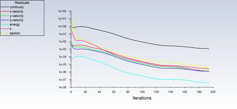
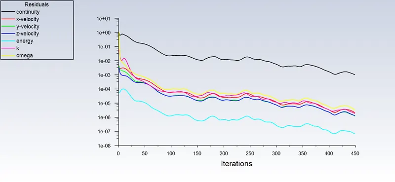
Approx. 194 iterations taken to converge solution. Approx. 449 iterations taken to converge solution.
Average weighted area Plot for Temp.:-
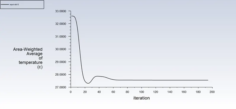
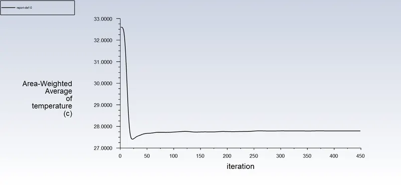
From the above snap outlet temp. of mixture is 27.55 degree C From the above snap outlet temp. of mixture is 27.79 degree C
Standard deviation plot:-
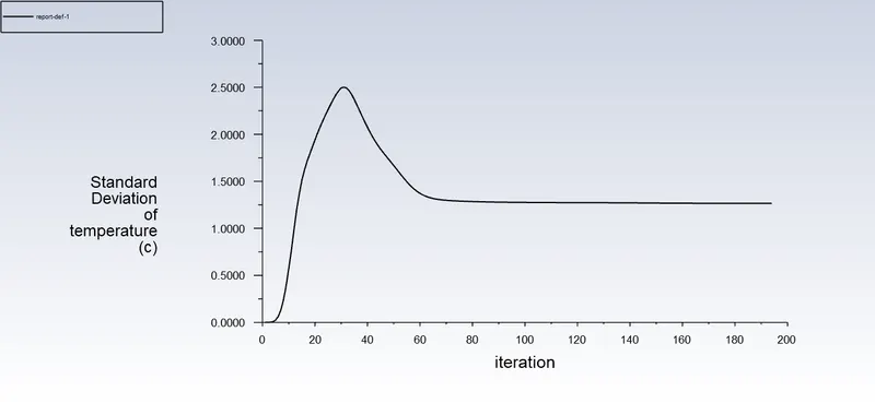
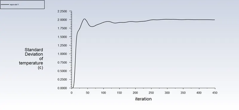
From the above snap standard deviation is 1.26 From the above snap standard deviation is 1.99
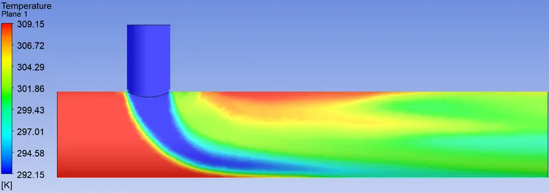
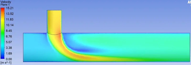
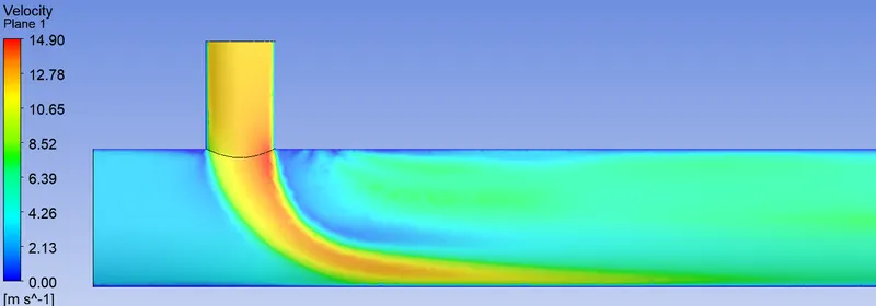
Contour plots:-
1) For Temp. distribution
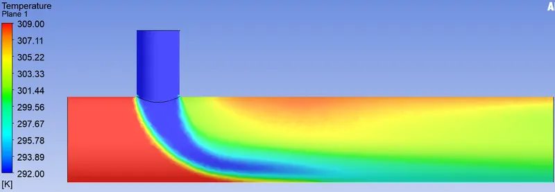
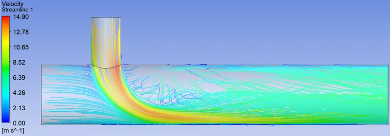
2) For Velocity. distribution
Line plots:-
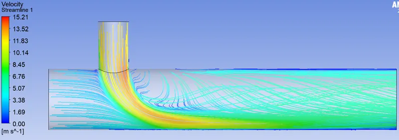
1) For Velocity. distribution
Summary:- Short Tee with MR=4
| K-epsilon | K-omega | |
| Cell count | 573264 | 573264 |
| Avg. Outlet Temp. | 27.55 degree C | 27.79 degree C |
| No. of Iterations | approx. 194 | approx. 449 |
| Standard deviation | 1.26 | 1.99 |
Conclusion:-
| K-epsilon(MR=2) | K-omega(MR=2) | K-epsilon(MR=4) | K-omega(MR=4) | |
| Cell count | 573264 | 573264 | 573264 | 573264 |
| Avg. Outlet Temp. | 30.4 degree C | 30.5 degree C | 27.55 degree C | 27.79 degree C |
| No. of Iterations | approx. 122 | approx. 250 | approx. 194 | approx. 449 |
| Standard deviation | 1.77 | 2.45 | 1.26 | 1.99 |
1) For MR 2 & 4, Standard deviation of k-epsilon model is lower than k-omega model. Hence k-epsilon model has better mixing efficiency than k-omega model.
2) For MR 2 & 4, k-epsilon model takes less number of iterations than k-omega model. Hence k-epsilon model is faster to converge solutions.
Hence we use k-epsilon model for future calcutions because it is more accurate & take less time to converge.
Case 2:- Long Tee
- Geometry Cleanup:-Import Long tee geometry into spaceclaim, spaceclaim gives various facility like CAD softwares, so we prepare geometry as per our simulation requirement.
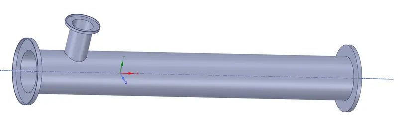
As per our simulation we are only interested in fluid flow analysis throught our long tee geometry, so we extract fluid volume from long tee geometry. Spaceclaim provide various option for extract the volume.
Goto Prepare -> Volume Extract -> Select edges
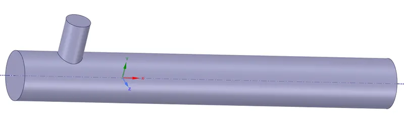
After extract flow volume, subpress for solid geometry so that it does not take part in mesh generation and futher simulation process.
b. Mesh Generation:-
In this step boundary naming also done. Boundary naming helps in for easy & correct visual of inlet/outlet and other geometry features so we can apply correct condition at correct place.
Mesh generation & element quality check is shown below-
we choose 1E-2 m element size.
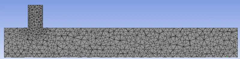
Goto Mesh -> Quality -> Mesh Metric -> Element Quality
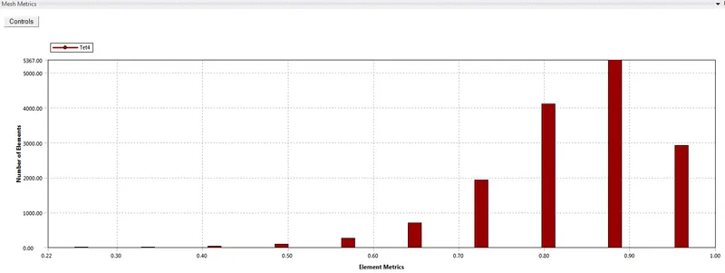
please check element quality should not be less than 5%.
c. Fluent Setup:-
At Fluent launcher choose Double precision option & solver process.
Condition 1:-
Long Tee with a hot inlet velocity of 3 m/s & Momentum ratio of 2
| SETUP | K-epsilon |
| Solver Type | Pressure Based |
| Velocity Formulation | Absolute |
| Time | Steady |
| Viscous Model | Realizable k-epsilon with standard wall function |
| Material | Air |
| Cell Zones | |
| Volume_Volume | Fluid type- Air |
| Inlet x (velocity inlet) | |
| Velocity Magnitude= 3 m/s | |
| Temp.= 36 degree C | |
| Boundaries | Inlet y (velocity inlet) |
| Velocity Magnitude= 6 m/s | |
| Temp.= 19 degree C | |
| Outlet (pressure outlet) | |
| Gauge Pressure= 0 pas. | |
| Walls= Stationary walls |
After placing all input condition solution is initialize by Hybrid Initialization.
d. Results:-
For k-epsilon model
Residuals plot:-
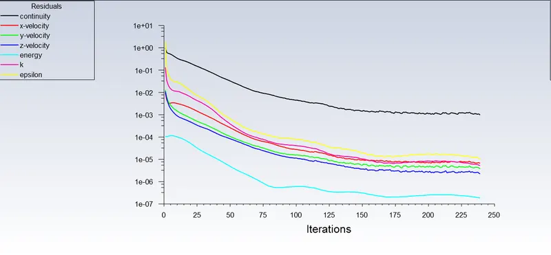
Approx. 239 iterations taken to converge solution.
Average weighted area Plot for Temp.:-
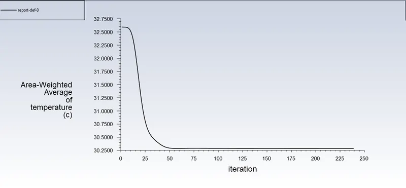
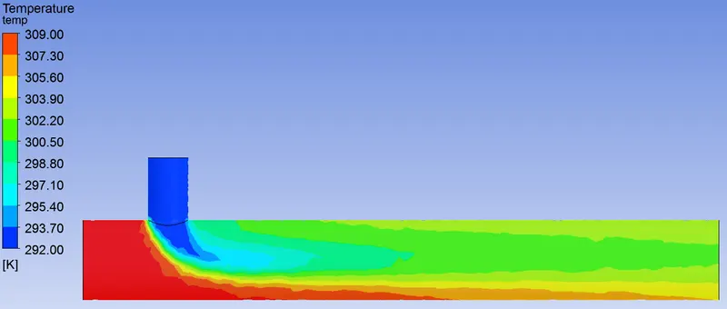
From the above snap outlet temp. of mixture is 30.28 degree C.
Standard deviation plot:-
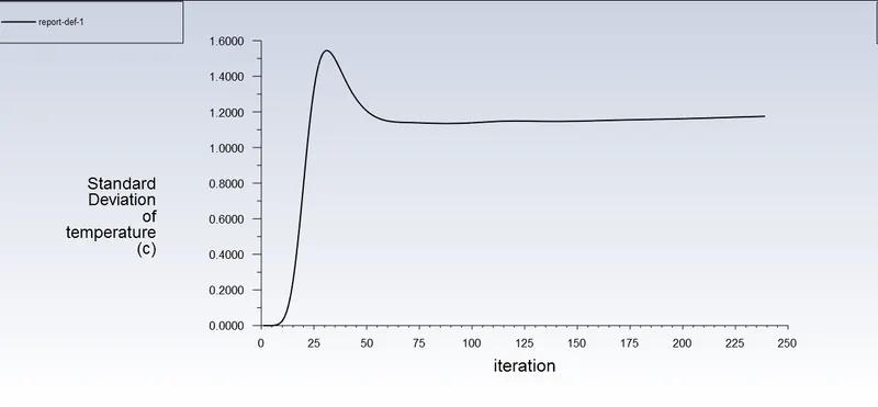
From the above snap standard deviation is 1.17
Contour plots:-
1) For Temp. distribution
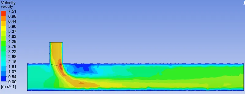
2) For Velocity. distribution
Line plots:-
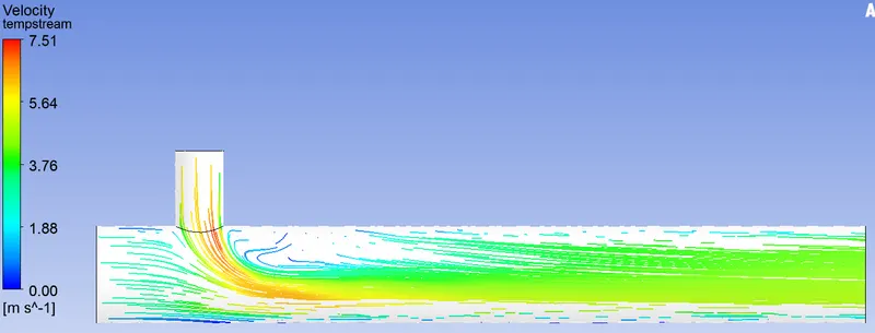
1) For Velocity. distribution
Summary:- Long Tee with MR=2
| K-epsilon | |
| Cell count | 15368 |
| Avg. Outlet Temp. | 30.28 degree C |
| No. of Iterations | approx. 239 |
| Standard deviation | 1.17 |
Long Tee with a hot inlet velocity of 3 m/s & Momentum ratio of 4
| SETUP | K-epsilon |
| Solver Type | Pressure Based |
| Velocity Formulation | Absolute |
| Time | Steady |
| Viscous Model | Realizable k-epsilon with standard wall function |
| Material | Air |
| Cell Zones | |
| Volume_Volume | Fluid type- Air |
| Inlet x (velocity inlet) | |
| Velocity Magnitude= 3 m/s | |
| Temp.= 36 degree C | |
| Boundaries | Inlet y (velocity inlet) |
| Velocity Magnitude= 12 m/s | |
| Temp.= 19 degree C | |
| Outlet (pressure outlet) | |
| Gauge Pressure= 0 pas. | |
| Walls= Stationary walls |
After placing all input condition solution is initialize by Hybrid Initialization.
d. Results:-
For k-epsilon model
Residuals plot:-
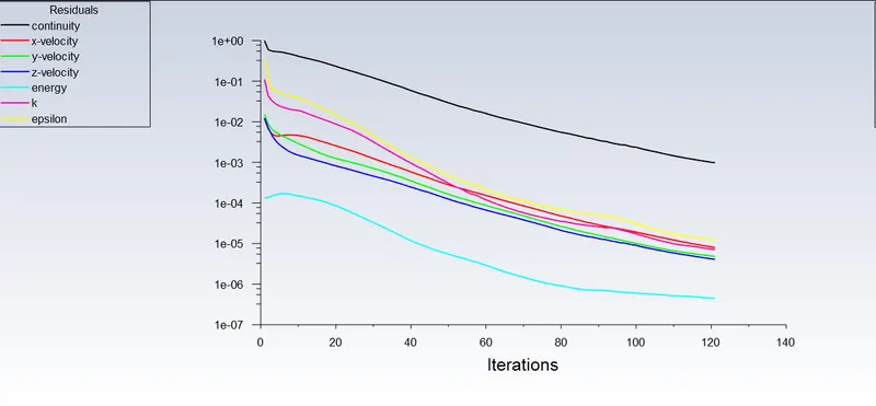
Approx. 121 iterations taken to converge solution.
Average weighted area Plot for Temp.:-
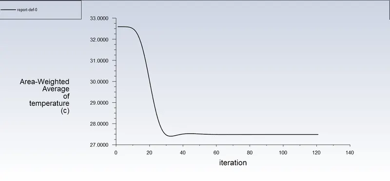
From the above snap outlet temp. of mixture is 27.49 degree C.
Standard deviation plot:-
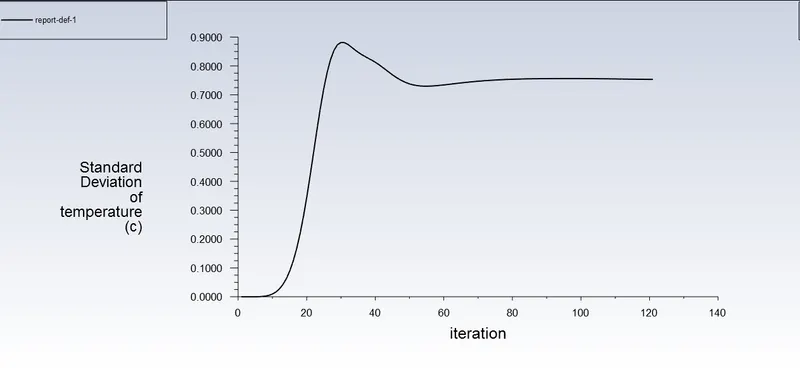
From the above snap standard deviation is 0.75
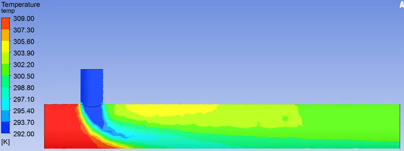
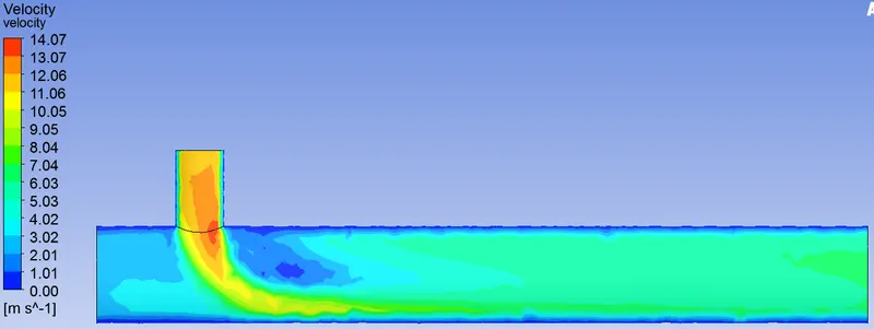
Contour plots:-
1) For Temp. distribution
2) For Velocity. distribution
Line plots:
1) For Velocity. distribution
Summary:- Long Tee with MR=4
| K-epsilon | |
| Cell count | 15368 |
| Avg. Outlet Temp. | 27.49 degree C |
| No. of Iterations | approx. 121 |
| Standard deviation | 0.75 |
| K-epsilon (MR= 2) | K-epsilon (MR= 4) | |
| Cell count | 15368 | 15368 |
| Avg. Outlet Temp. | 30.28 degree C | 27.49 degree C |
| No. of Iterations | approx. 239 | approx. 121 |
| Standard deviation | 1.17 | 0.75 |
Conclusion:-
| Short Tee | Long Tee | |||
| K-epsilon(MR=2) | K-epsilon(MR=4) | K-epsilon(MR=2) | K-epsilon(MR=4) | |
| Cell count | 573264 | 573264 | 15368 | 15368 |
| Avg. Outlet Temp. | 30.4 degree C | 27.55 degree C | 30.28 degree C | 27.49 degree C |
| No. of Iterations | approx. 122 | approx. 194 | approx. 239 | approx. 121 |
| Standard deviation | 1.77 | 1.26 | 1.17 | 0.75 |
1) As we see in above table long tee outlet temp. is approx similar to short tree in respective MR, hence longer length does not have significant effect on efficiency of mixing tee.
2) The tee mixing effectiveness increases when the velocity of the cold inlet fluid increases. Hence MR 4 has better effectiveness than 2.
3) From the grid independence test, we can conclude that the finer the size mesh, the better the accuracy of the solution. Hence at the finer grid size, we got better mixing efficiency. But at the same time, computional time increases significantly.