Flow Over a Backward Facing Step

Flow Over a Backward Facing Step

Aim: To perform flow over a backward facing step simulation using Converge-CFD and postprocess the result in Paraview.

Objective:

Run 3 simulations and compare the results between all the 3 simulations.

3 different base mesh sizes are,

• dx = 2e-3m, dy = 2e-3m, dz = 2e-3m
• dx = 1.5e-3m, dy = 1.5e-3m, dz = 1.5e-3m
• dx = 1.0e-3m, dy = 1.0e-3m, dz = 1.0e-3m

Procedure:

Backward-facing step is a standard geometry used for visualizing the recirculation flow and validating turbulence models. BFS flow is one representative model for seperation flows, which is widely used in aerodynamic flows,condensers, vehicles etc. For this case backeard facing step is constructed using triangle commands on converge.

• Before setting up the simulation download necessary softwares that are required for simulation and post processing.
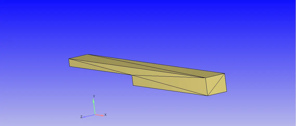
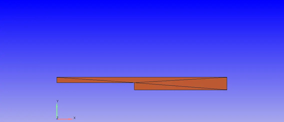
• Initially open Converge Studio and create geometry of a Channel. Create geometry as per the dimensions.
• Next go to Geometry > options > select Surface Normal. After selecting the S.Normal the normals point towards outside, so selec any one arrow that is point outwards and clik on them. Then the normals change their direction to inwards.
• After setting the geometry, next important thing is to diagnosis the geometry for errors/problems. For this go to Right Bottom side, select Diagnosis > click on All intersections > click Find. On top we can check for problems in Problem Triangles.
• Now if there are no errors found then the geometry is correct.
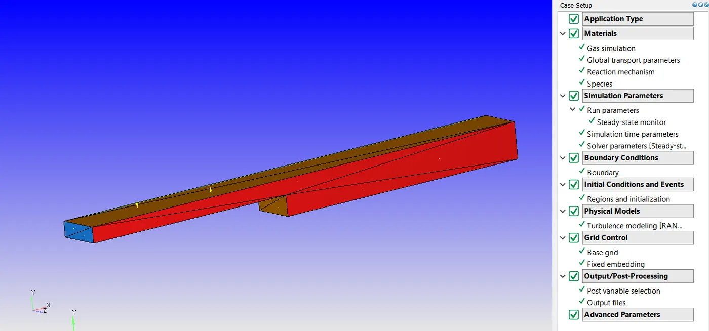
• To we should do Case Setup. Just beside Diagonisis > click on Cae Setup > in case setup window we can see 'Begin Case Setup" > click on it to set the setup.

Case Setup:

Application Type = Time-based

Materials -

Predefined mixtures = Air

Select 'Gas Simulation' & 'Species(not in mech.dat)'

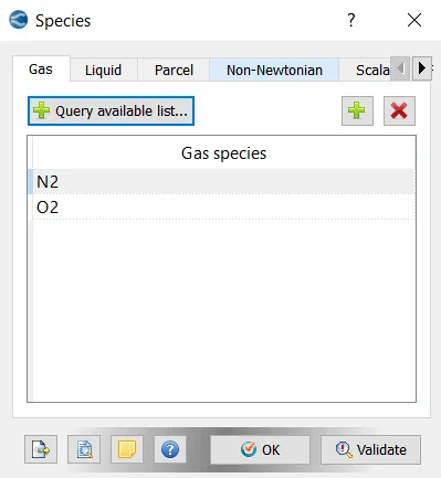
> Click on Species > select Gas > click on Add and select N2 &O2.

Simulation Parameters-

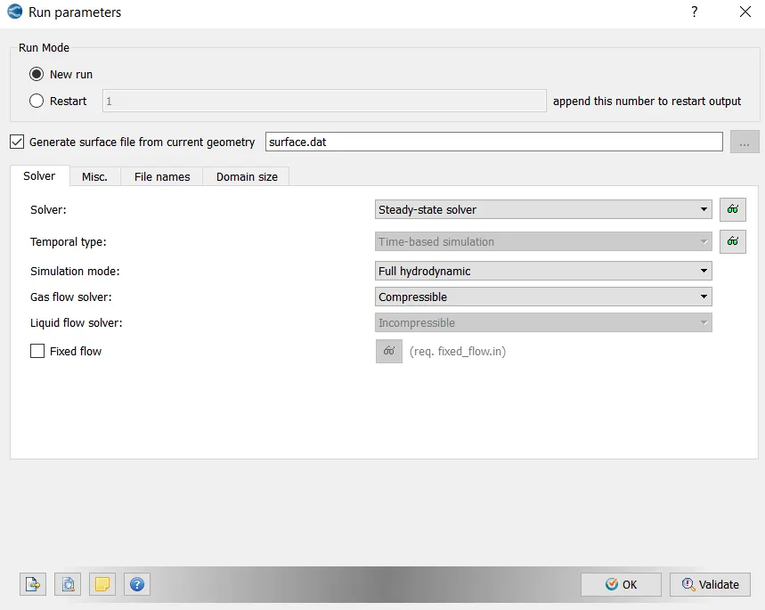
In Run Parameters two main things to be considered:-

(a.) select the following solver settings

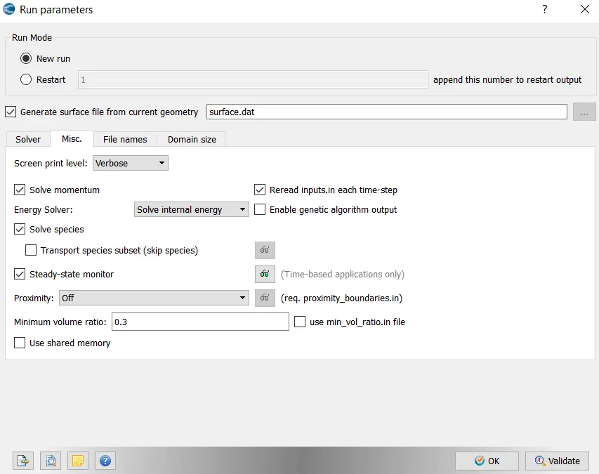
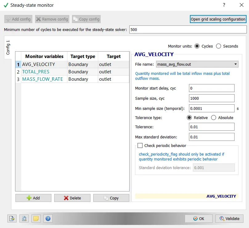
(b.) Go to Misc. > uncheck UseSharedMemory and click on Steady-State Monitor .

Steady-State Monitor:-

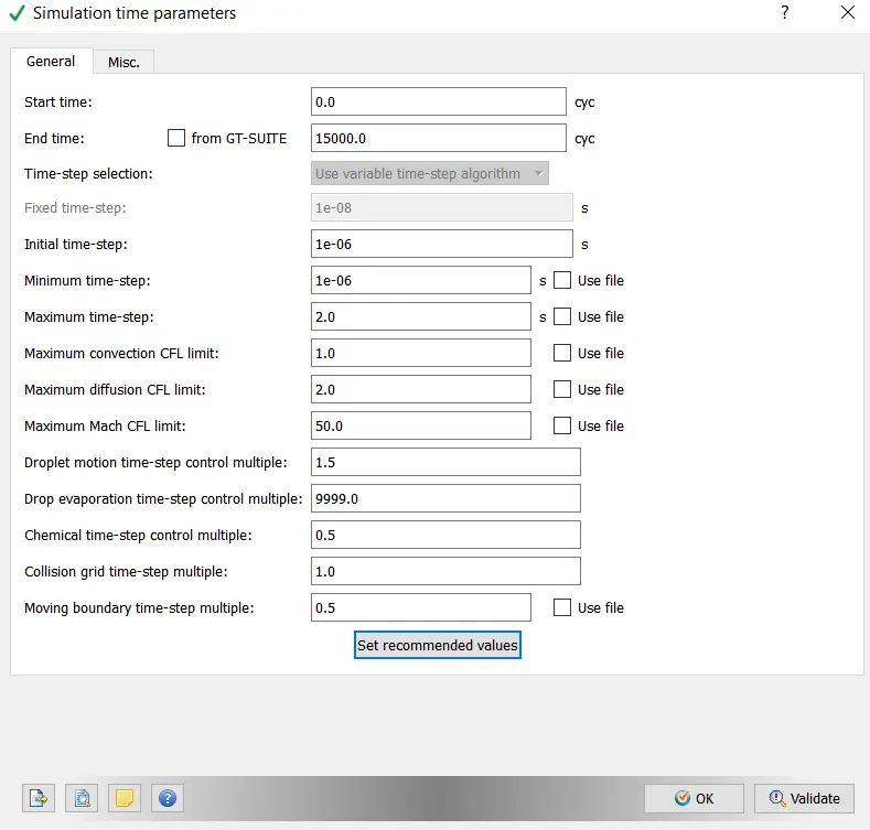
Simulation Time Parameters-

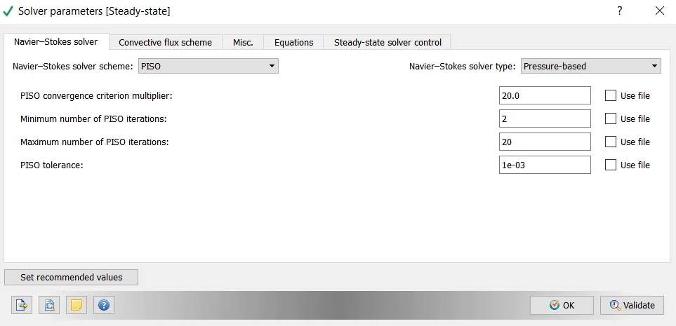
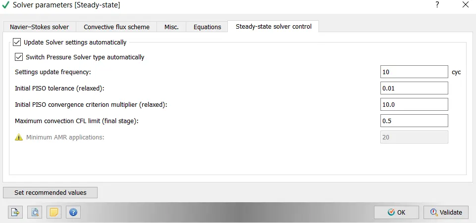
Solver Parameters [Steady-State]-

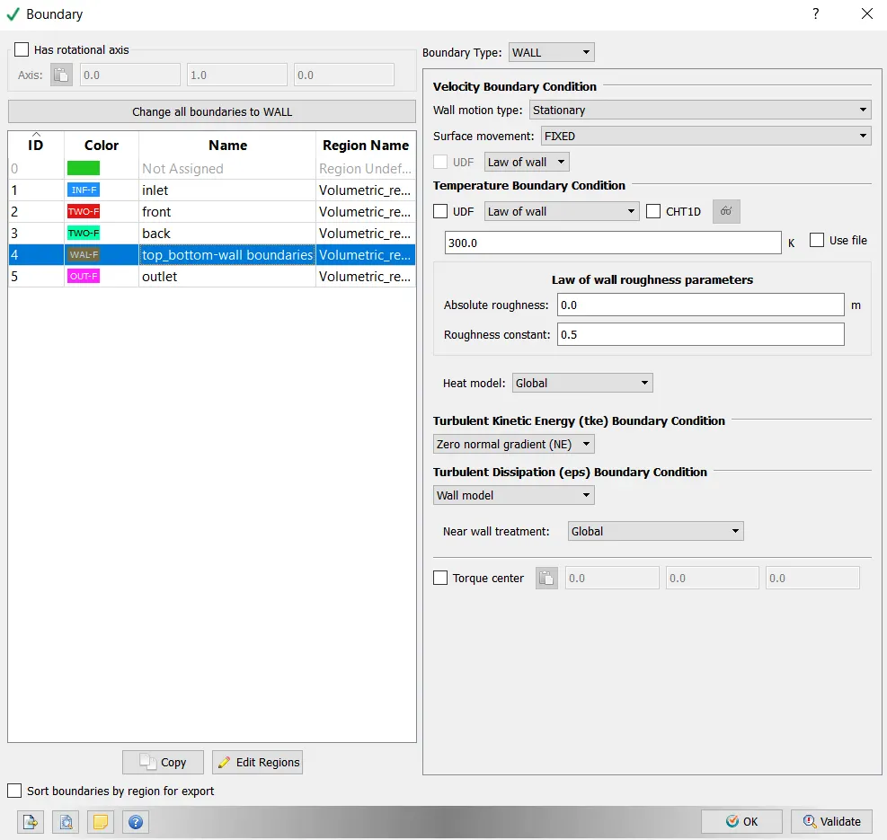
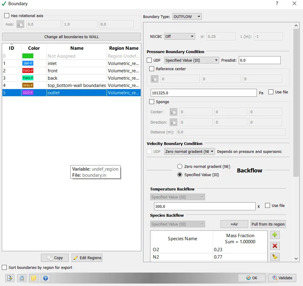
Boundary Conditions-

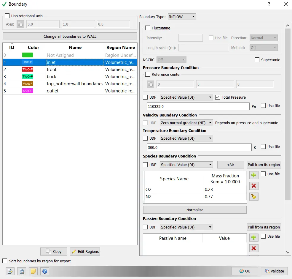
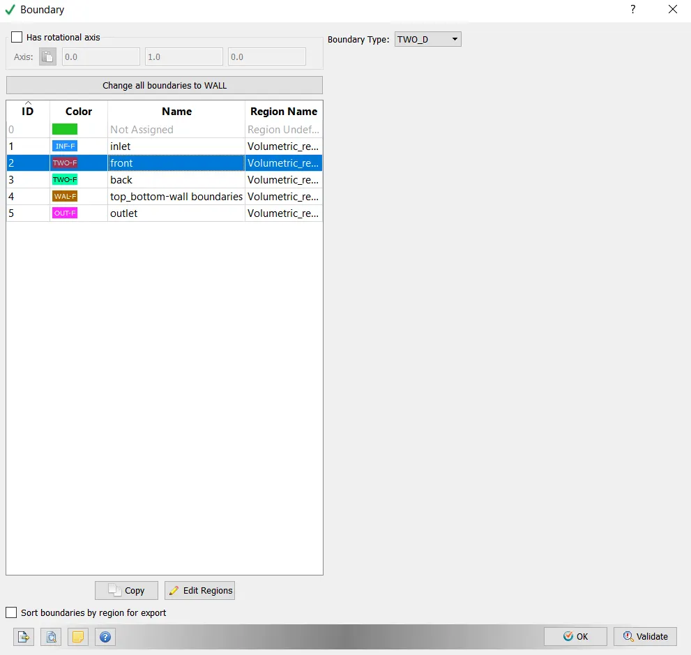
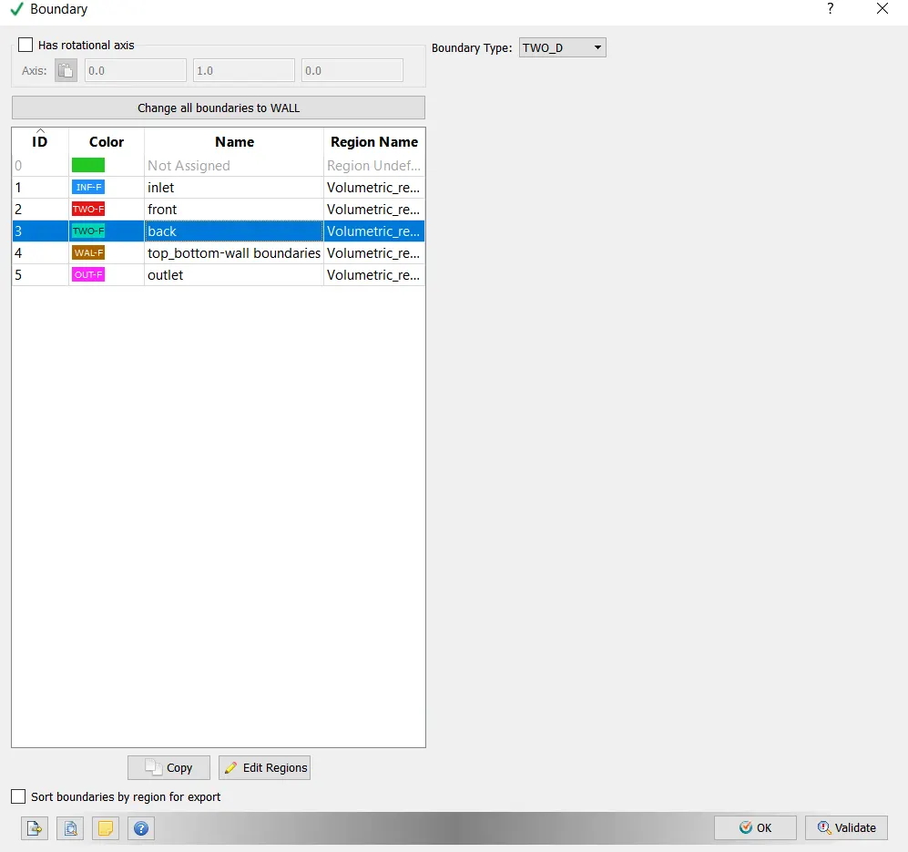
Booundary:

Initial Conditions and Events:-

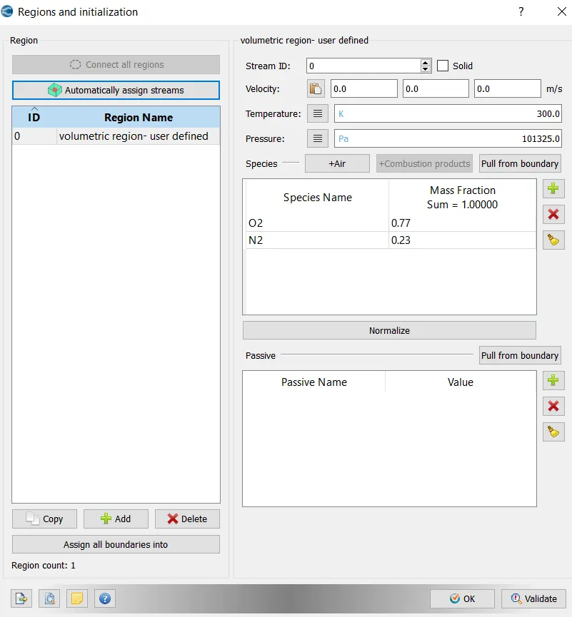
Regions and Initialization:

Physical Models:-

Uncheck Turbulence Modeling in this case.

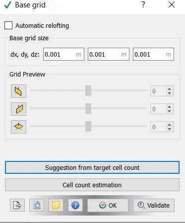
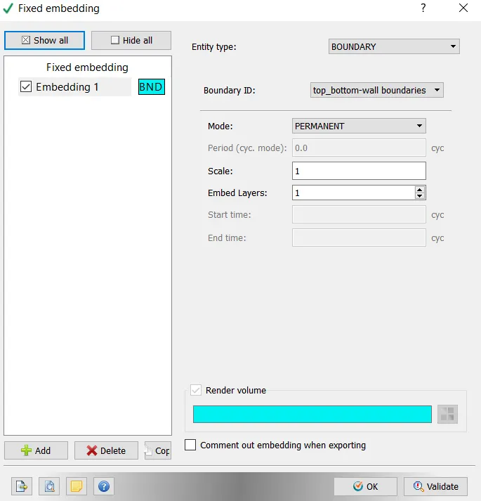
Grid Control:-

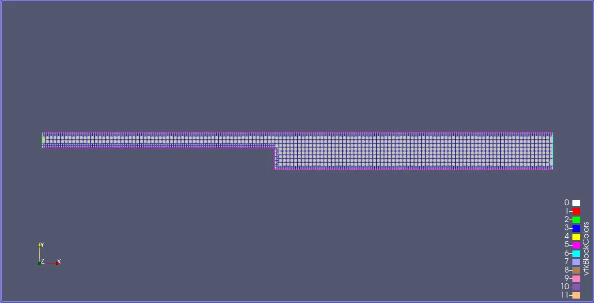
Base Grid:

case-1 dx = 2e-3m, dy = 2e-3m, dz = 2e-3m

case-2 dx = 2e-3m, dy = 2e-3m, dz = 2e-3m

case-3 dx = 1.0e-3m, dy = 1.0e-3m, dz = 1.0e-3m

Post-Processing:-

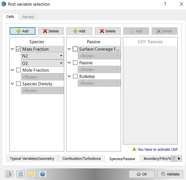
Post Variable Selection:

Click on Typical Variables/Geometry > Select required variables.

Click on Species/Passive

Output Files:

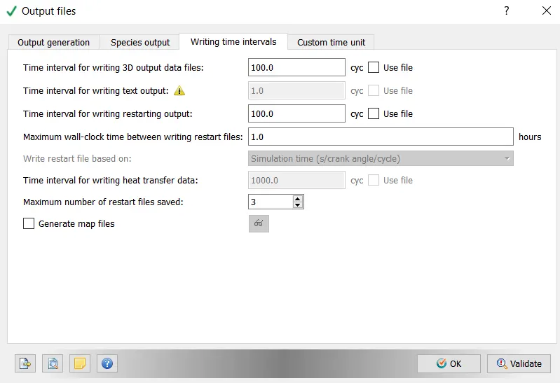
• With this setting up of the case is completed.
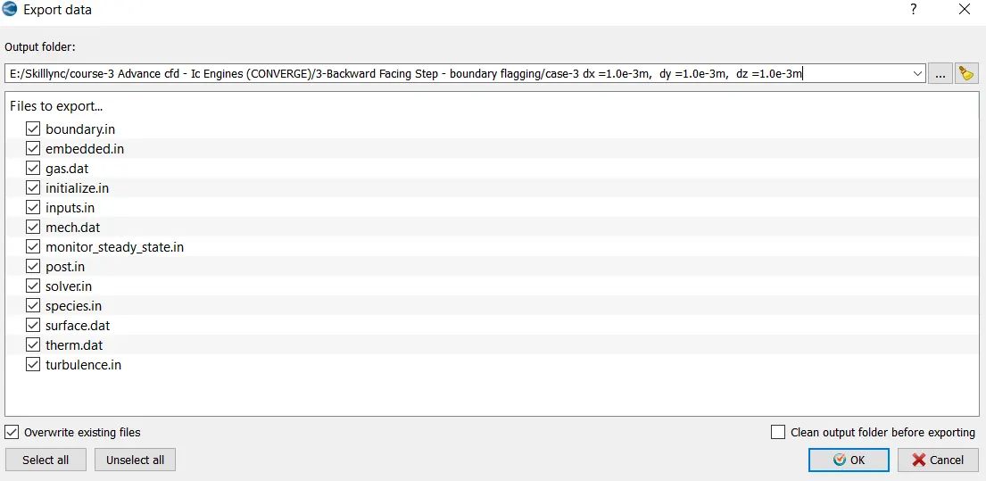
• Now go to File > Export > click on Export Input Files. select the destination folder(test) to save the data.

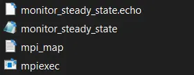
• After importing the input files, paste the "mpiexec.exe file".

• Now open Cygwin and navigate to the location where the setup files are imported.

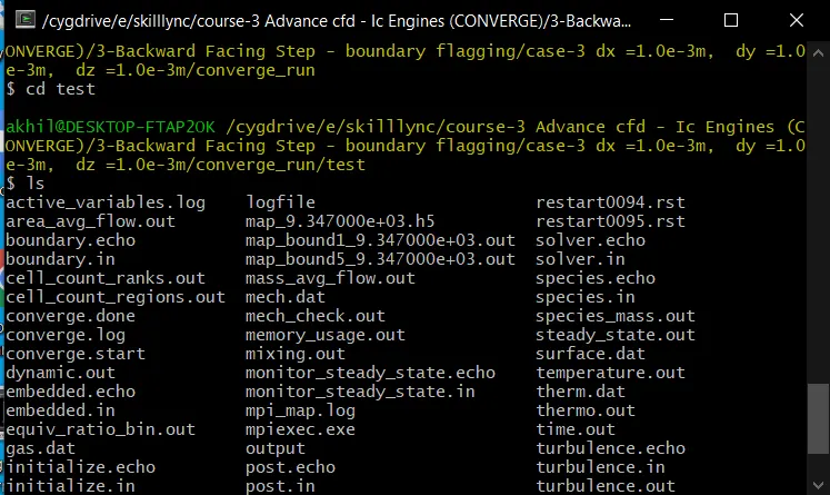
• Once we navigate to the respective folder, we need to run the simulation. To run the simulation use the following command in Cygwin;

>> Here path is copied from " C:ProgramFilesConvergent_ScienceCONVERGE3.0.15binconverge-intelmpi.exe ".

• Now the simulation starts running , and it displays the steps in cygwin. As the simulation begins it creates multiple folders (i.e. '.scratch' & output) in the path where we saved the input files.
• Once the simulation is complete, to perform post processing we need to convert the obtained result data into format where we can access in Paraview. These converted files are directed to the Output folder.

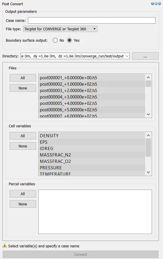
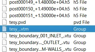
• Open PARAVIEW > direct to folder where the output is saved > select '.vtm(group file)' > data imported to paraview.

• Necessary contours, profiles and animations are generated using paraview. To generate plots we can use ConvergeStudio (line plotting option).
• Hence required plots, contours , animations are obtained in order to study the results.

Geometry:

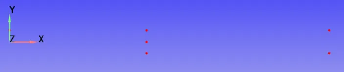
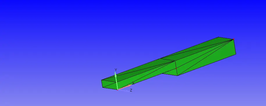
Case Setup:

Observations:

Case-1

Mesh sizes - dx =2e-3m, dy =2e-3m, dz =2e-3m

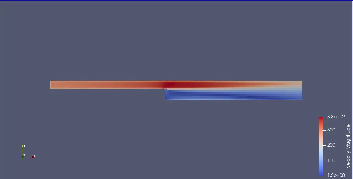
Velocity Contour:

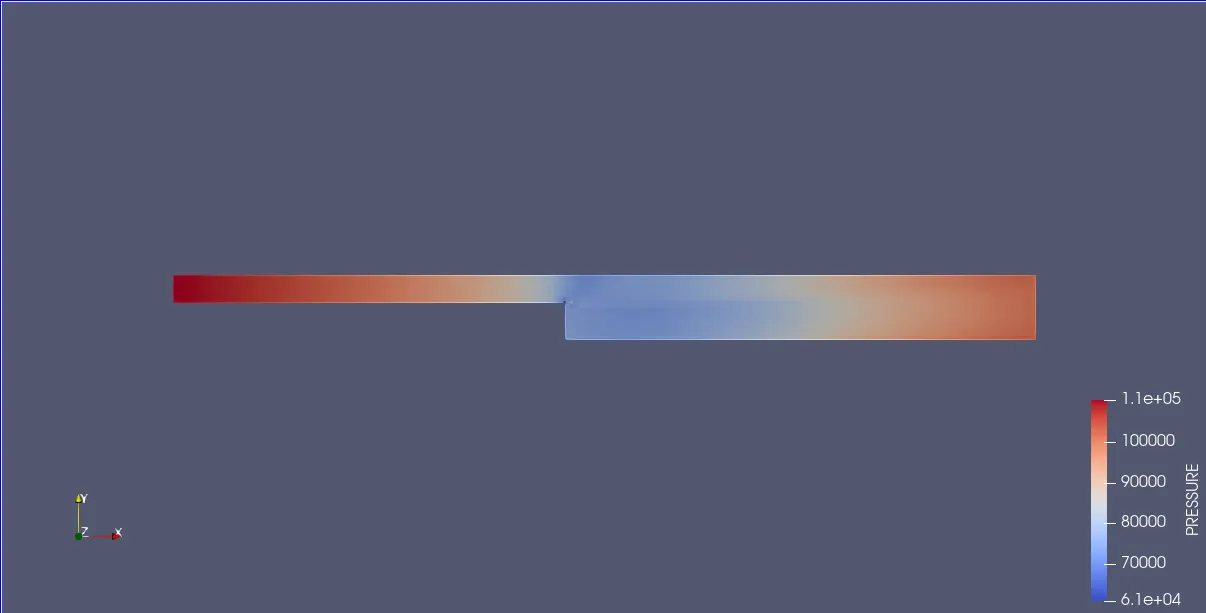
Pressure Contour:

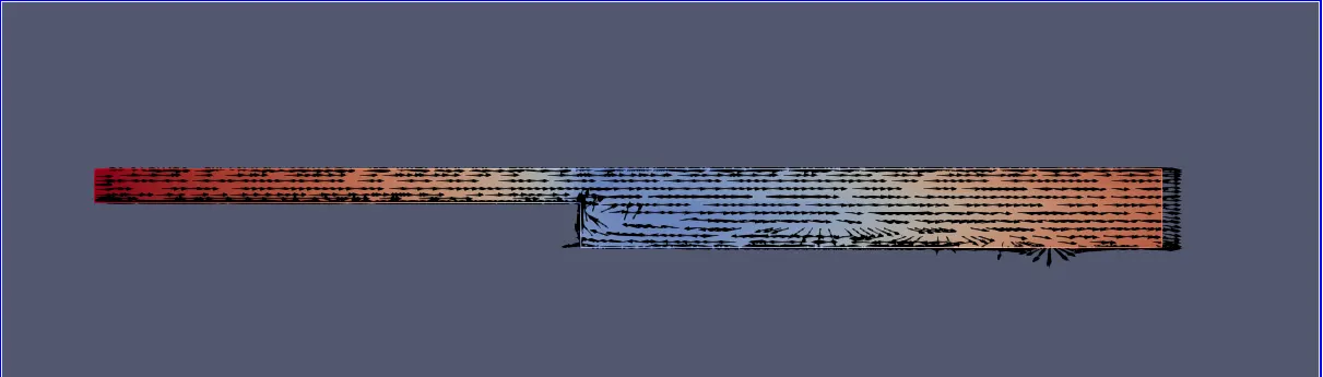
Velocity vectors:

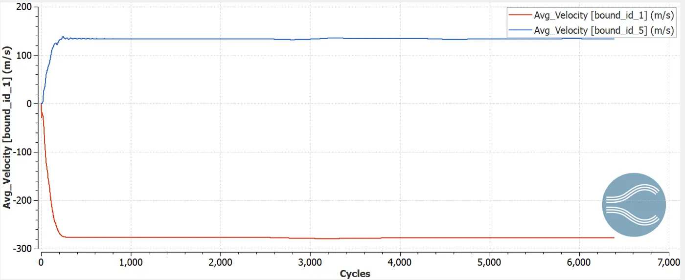
Velocity Plot:

Pressure Plot:

Mass Flow Rate plot:

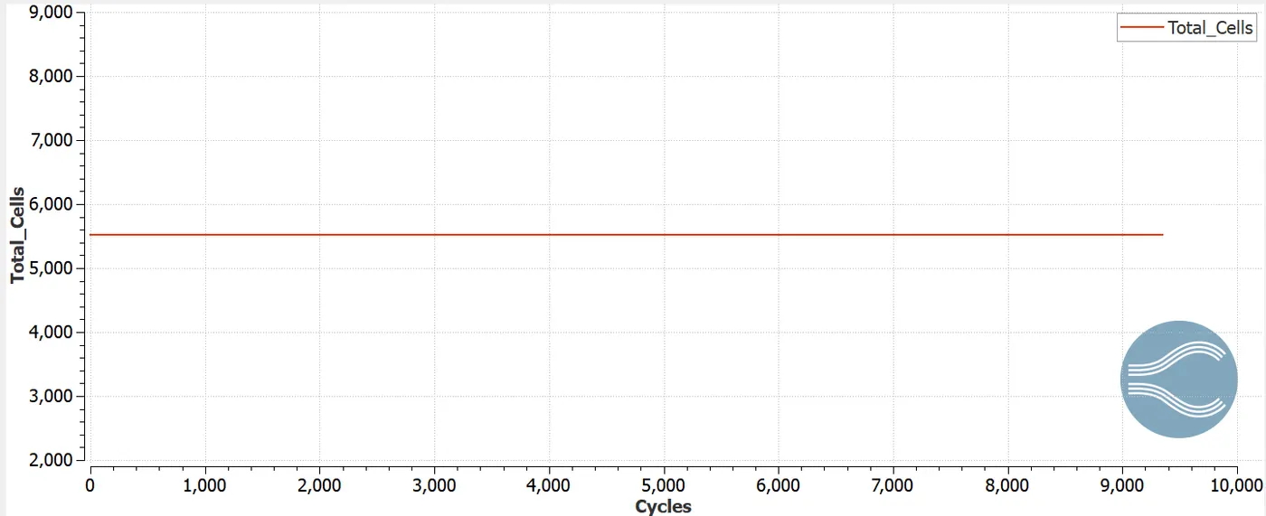
Cell Count plot:

Animation:

Velocity:

Pressure:

Case-2

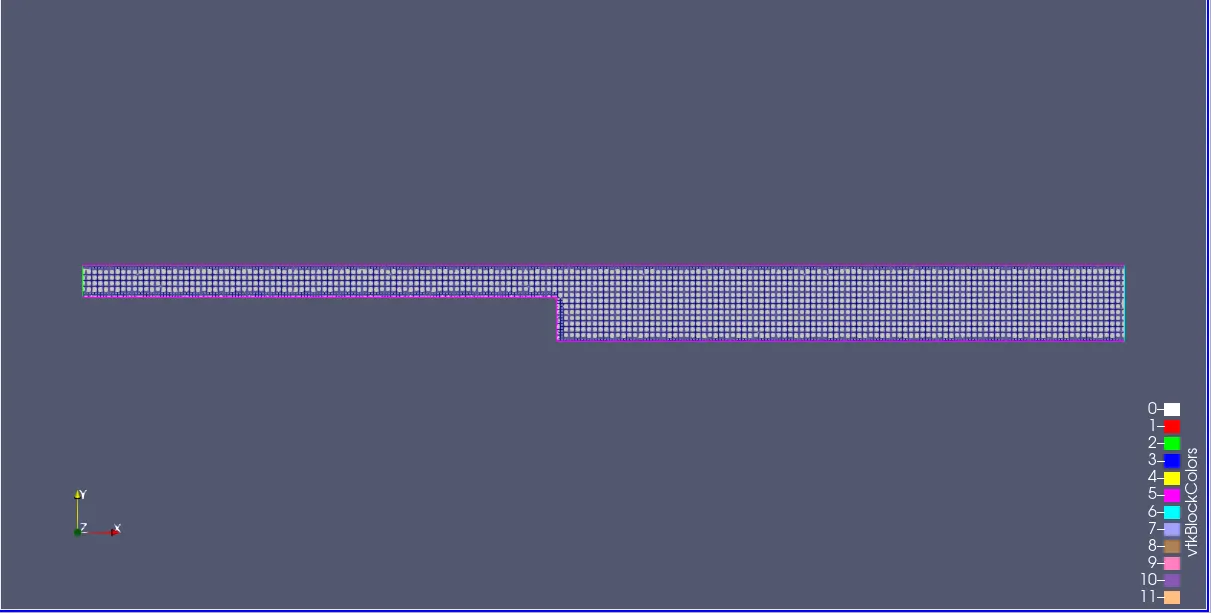
Mesh sizes - dx =1.5e-3m, dy =1.5e-3m, dz =1.5e-3m

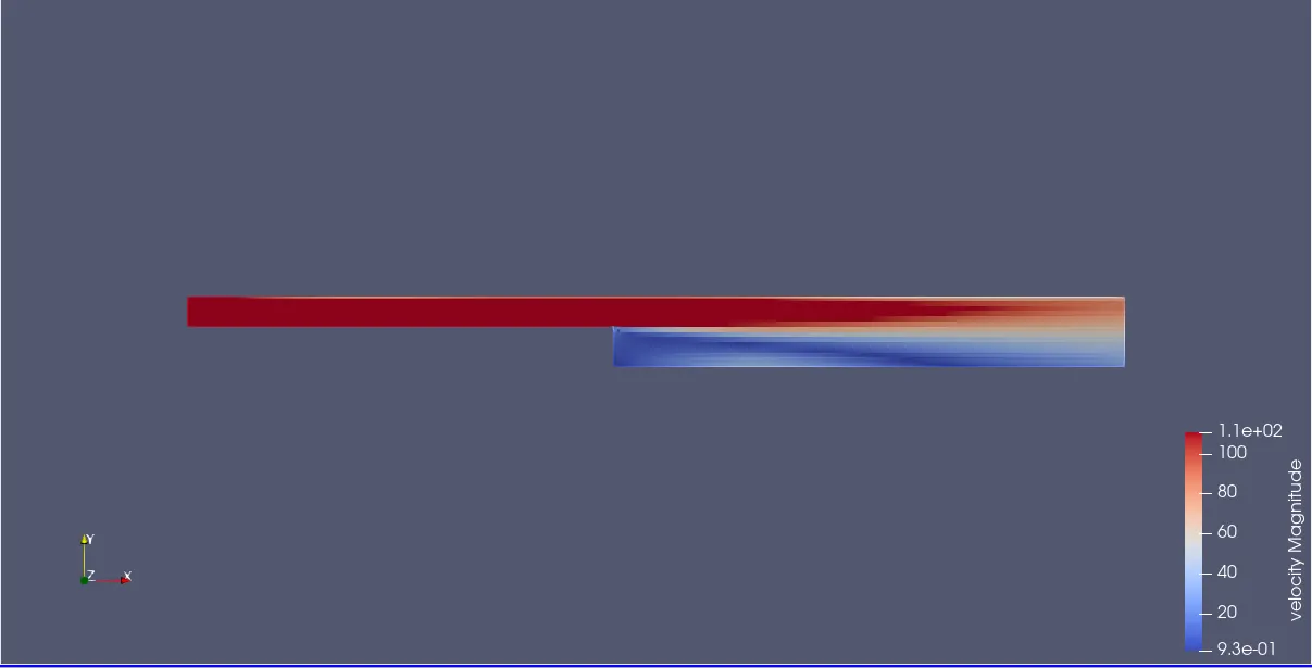
Velocity Contour:

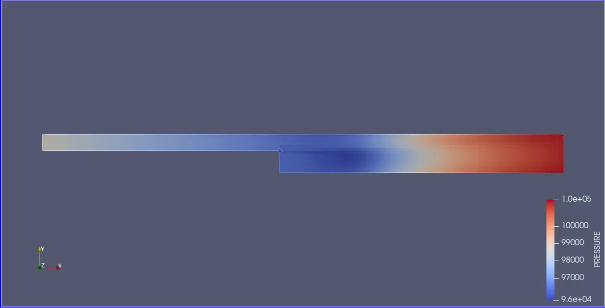
Pressure Contour:

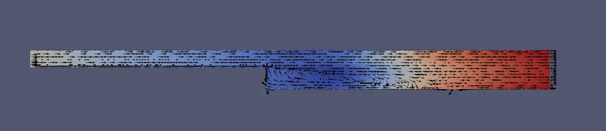
Velocity vectors:

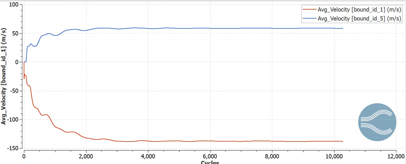
Velocity Plot:

Pressure Plot:

Mass Flow Rate plot:

Cell Count plot:

Animation:

Velocity:

Pressure:

Case-3

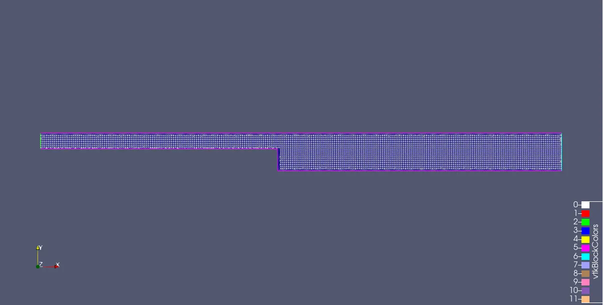
Mesh sizes - dx =1.0e-3m, dy =1.0e-3m, dz =1.0e-3m

Velocity Contour:

Pressure Contour:

Velocity vectors:

Velocity Plot:

Pressure Plot:

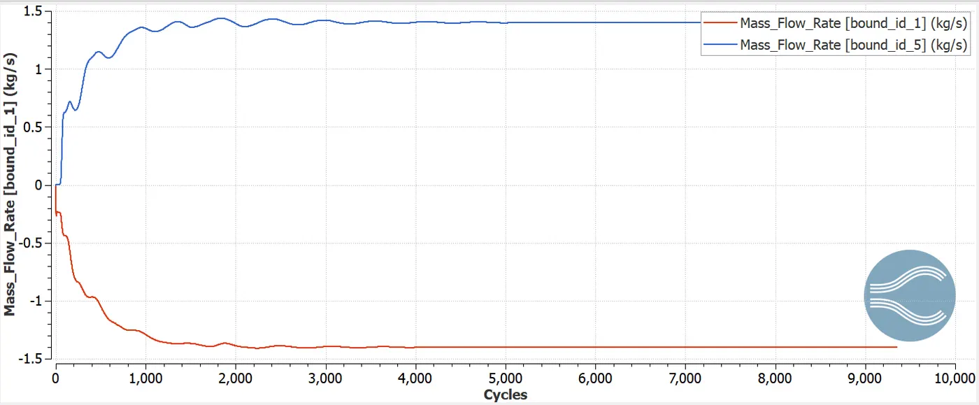
Mass Flow Rate plot:

Cell Count plot:

Animation:

Velocity:

Pressure:

Results:

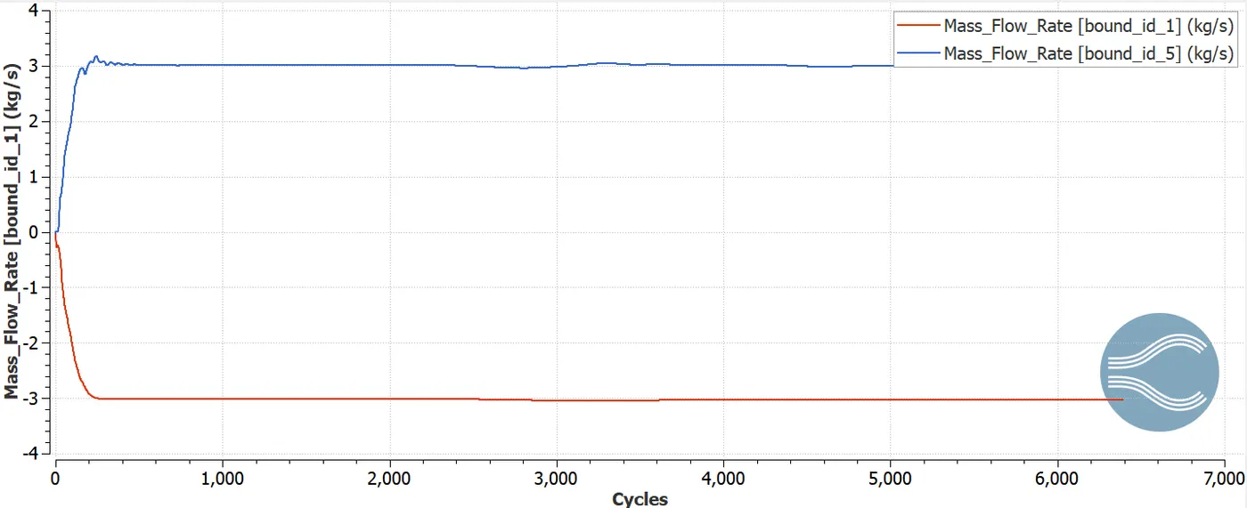
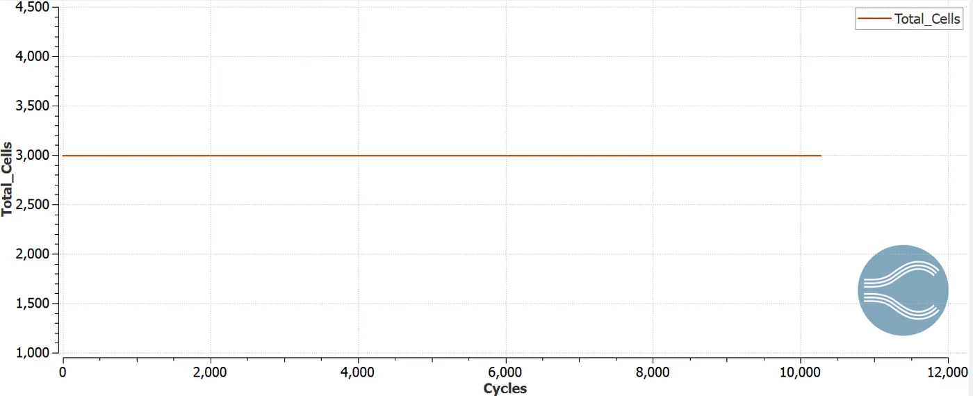
• From the simulations performed it is clear that, for mesh size (2e-3, 1.5e-3, 1.0e-3) the total cell count is increased by refining the mesh finer. If the mesh becomes finer and finer the total cell count also increases , as the cell count increases the computational time also increases.
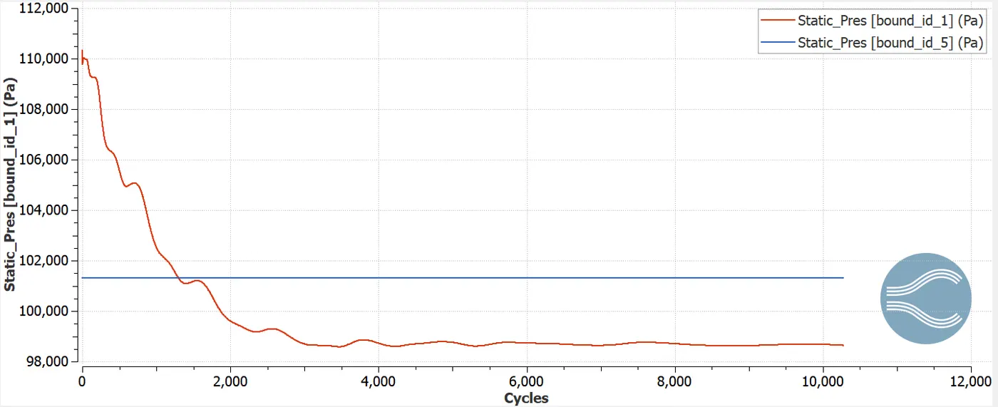
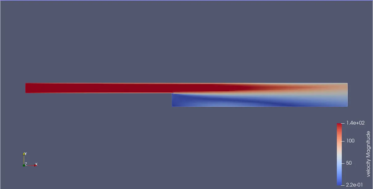
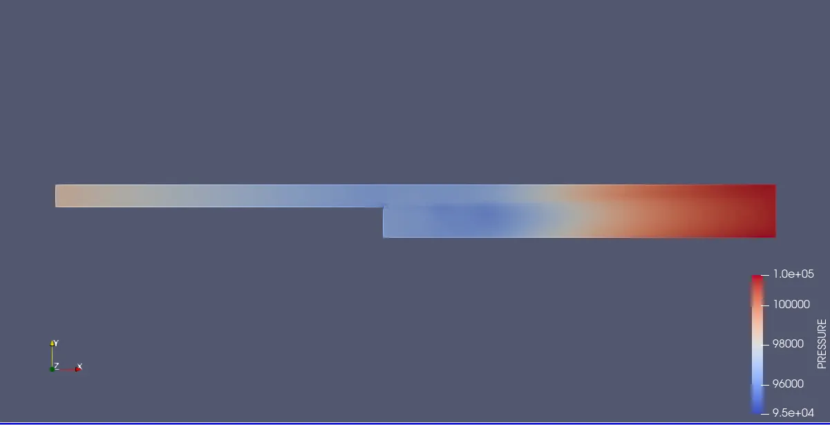
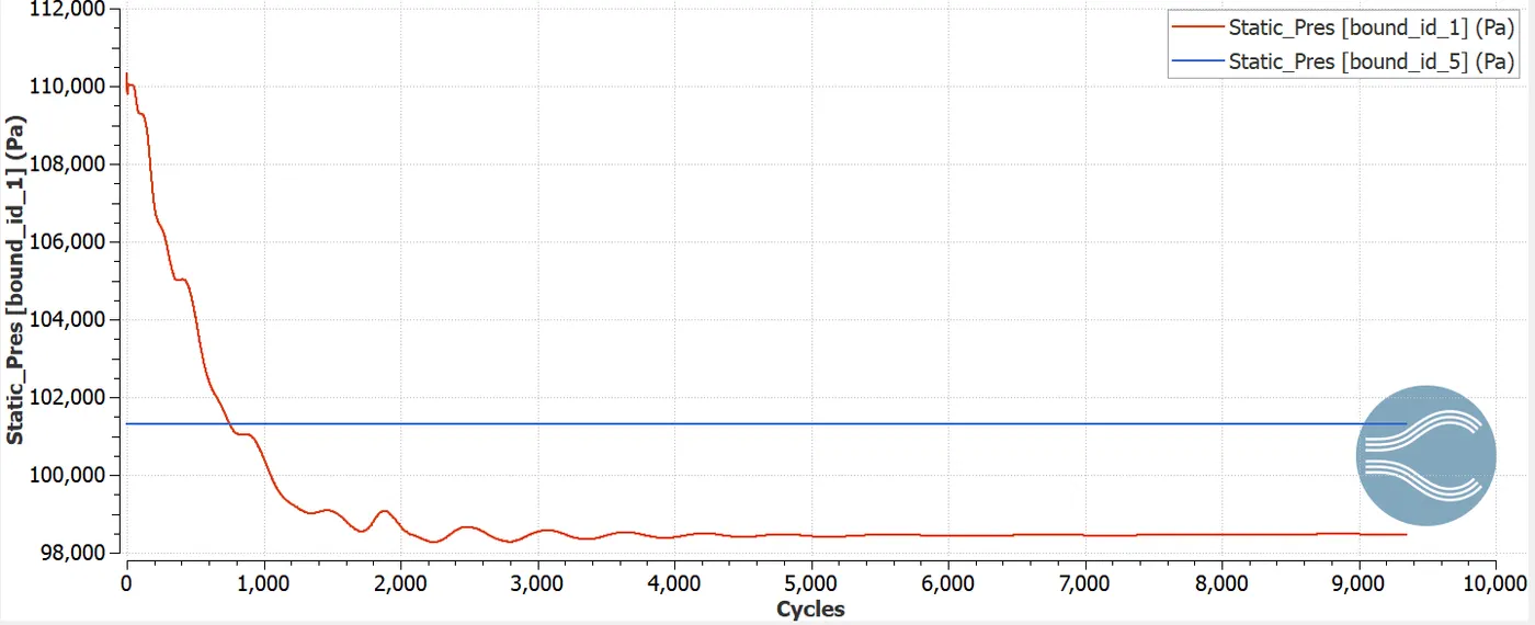
• From pressure contours, it is clear that static pressure is constant at the outlet boundary but decreases in the inlet boundary.
• Static pressure reduces at the inlet , due to excessive momentum loss near the step wall the flow seperates resulting a zone with pressure gradient called as recirculation zone. The velocity vector plot clear shows the recirculation zone in all the cases.
• Near the step in the geometry, we can see the seperation of the flow. this is due to effect of boundary layer seperation. Due to this there will be disturbance in pressure and velocity.At this point fluid seperates and tends to recirculate.
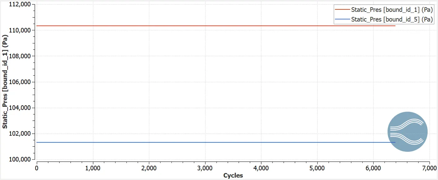
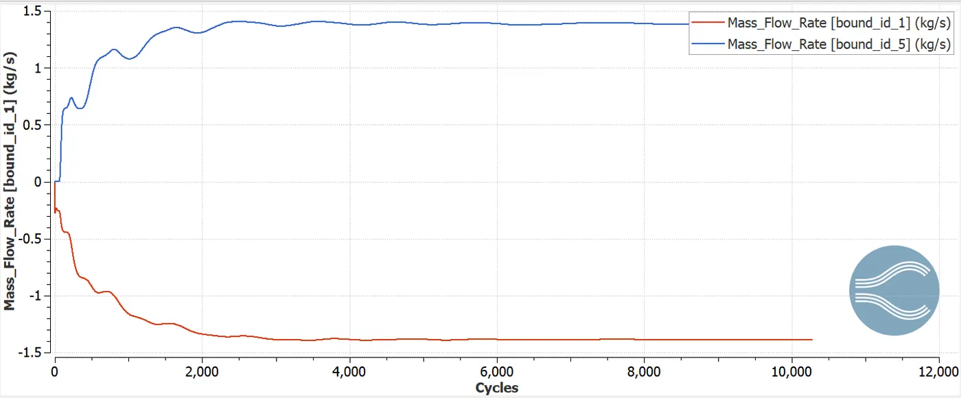
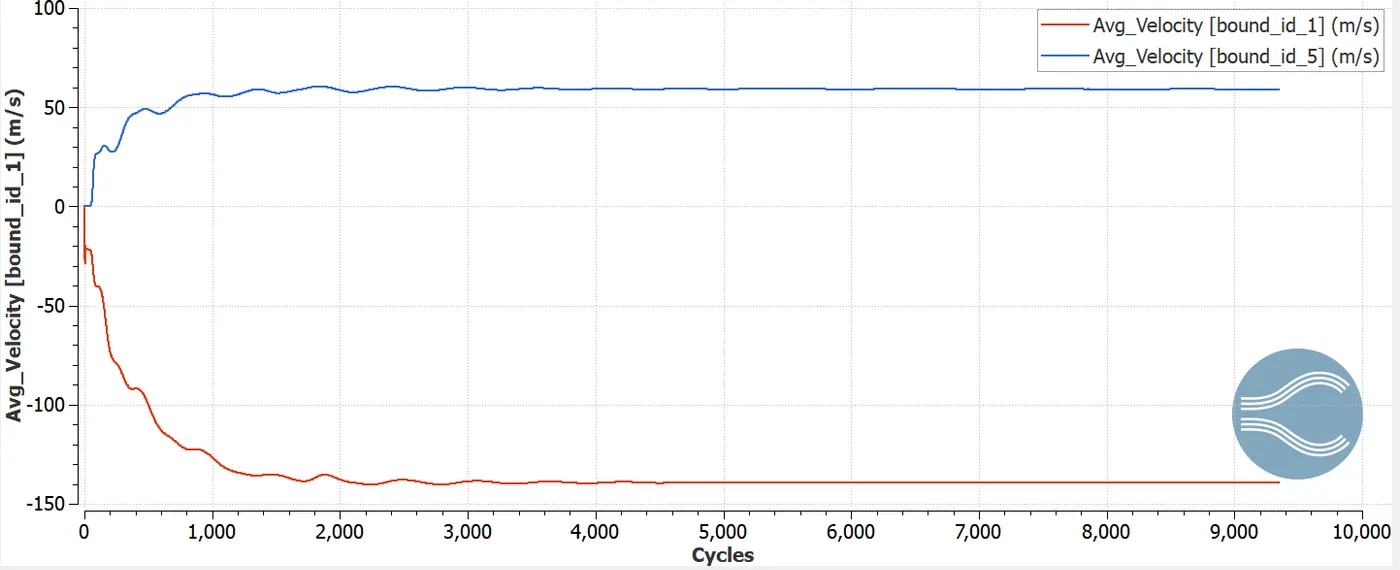
• Mass Flow Rate at the outlets for the refined cases are almost same.When both inlets and outlets are compared we can observe a positive flow and a negative flow.
• It is observed that, velocity in the initial case is highest but as the mesh is coarse it is generally not preffered to be accurate. In the next two cases it calculated more accurately.

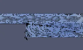
In the above vector plot, it is seen that some vectors are not in the direction of the flow. This mainly happens because of change in area. Near the step in the geometry, we can see the seperation of the flow. this is due to effect of boundary layer seperation.Due to the change in area there is a pressure drop, which leads to the seperation of the flow. The boundary layer seperation is a phenomenon which occurs when fluid experiances a sudden change in area or the path of the flow.

Conclusion:

The flow over a backward facing step using Converge CFD is performed. With different mesh sizes the accurate results are obtained. Various plots, contours, animations are generated. Also studied how the seperation of flow is taking place from the results obtained.