Final Project: Electric Rickshaw modelling

FINAL PROJECT

ELECTRIC RICKSHAW MODELLING

Create a detailed MATLAB model of an electric rickshaw (three-wheel passenger vehicle) as per details below:

Rear wheels driven by PM brushed type motor

Assume efficiency points of motor controller and motor

Make an excel sheet of all input and assumed data

Results: For any three standard driving cycles show energy consumption, temperature rise of motor and controller for 100 km constant speed driving at 45 kmph.

Objective: To create a MATLAB model of electric rickshaw using a Battery and PMDC motor and discussing in detail about the

• System level configurations
• Model parameters
• Results
• Conclusion

Electric Vehicle: An All-electric vehicle also called a Battery Electric Vehicle (BEV), uses one or more electric motors instead of an internal combustion engine. The vehicle uses a large traction battery pack to power the electric motor and must be plugged in to a wall outlet or charging equipment, also called electric vehicle supply equipment (EVSE). Because it runs on electricity, the vehicle emits no exhaust from a tailpipe and does not contain the typical liquid fuel components, such as a fuel pump, fuel line, or fuel tank.

Key Components of an All-Electric Vehicle

EVs have 90% fewer moving parts than an ICE (Internal Combustion Engine) car.

Battery: Store the energy required to run an EV. The higher the rating of the battery, the higher the range.

Electric Motor: Using power from the battery pack, this motor drives the vehicle's wheels. Some vehicles use motor generators that perform both the drive and regeneration functions.

Power electronics controller (Inverter): This unit manages the flow of electrical energy delivered by the traction battery, controlling the speed of the electric traction motor and the torque it produces.

Charge port: The charge port allows the vehicle to connect to an external power supply in order to charge the battery pack.

Onboard charger: Takes the incoming AC electricity supplied via the charge port and converts it to DC power for charging the traction battery. It also communicates with the charging equipment and monitors battery characteristics such as voltage, current, temperature, and state of charge while charging the pack.

Thermal system (cooling): This system maintains a proper operating temperature range of the engine, electric motor, power electronics, and other components.

Transmission (electric): The transmission transfers mechanical power from the electric motor to drive the wheels.

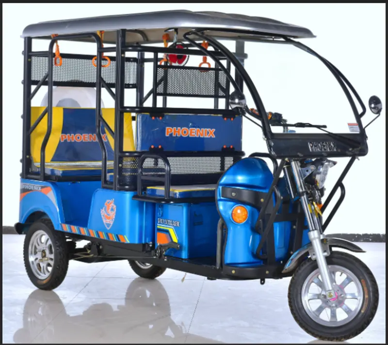
Vehicle Modelling:

• In order to be able to estimate the performance of an electric vehicle, it is very important to have a proper model of it.
• The electric vehicle model is very complex as it contains many different components. Each component needs to be modelled properly in order to prevent wrong conclusions.
• The design or rating of each component is a difficult task as the parameters of one component affect the power level of another one.
• There is therefore a risk that one component is rated inappropriately which may make the vehicle unnecessarily expensive or inefficient. Therefore, System level configurations are necessary.

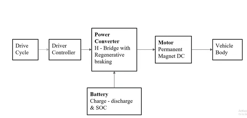
Block-Diagram:

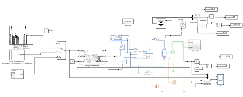
Simulink Model of Electric Vehicle:

Simulink Blocks used:

1. Drive Cycle Source
2. Longitudinal Driver
3. Controlled PWM voltage
4. Constant Voltage Source
5. H-Bridge
6. DC Motor
7. Vehicle Body
8. Tire (Magical Formula)
9. Simple Gear
10. Current Sensor
11. Controlled Current Source
12. Battery
13. Electrical Reference
14. Mechanical Rotational Reference
15. Multiport Switch
16. Integrator
17. Divide
18. Bus Selector
19. Constant
20. Display
21. Scope
22. Solver
23. PS-Simulink Converter
24. Power gui
25. From Workspace

System Level Modelling of Eelectric Rickshaw

Assumed Parameters:

S.No.	Parameters	Value
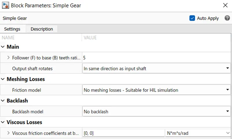
1	Rated DC Supply Voltage	300V
2	Rated load of Motor	10kW
3	PWM frequency	5000Hz
4	Output Voltage Amplitude	5V
5	Input voltage for 100% Duty cycle	1V
6	Gear ratio	5
7	Gross Weight of vehicle	400kg
8	Frontal area	2 sq.mtr
9	Drag coefficient	0.3
10	Air density	0.6 kg/m3
11	Rolling resistance	0.015
12	Battery Capacity	150 Ah

Vehicle Body

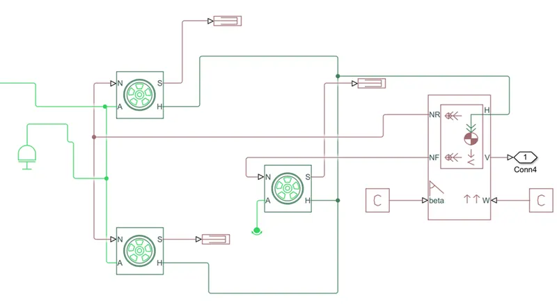
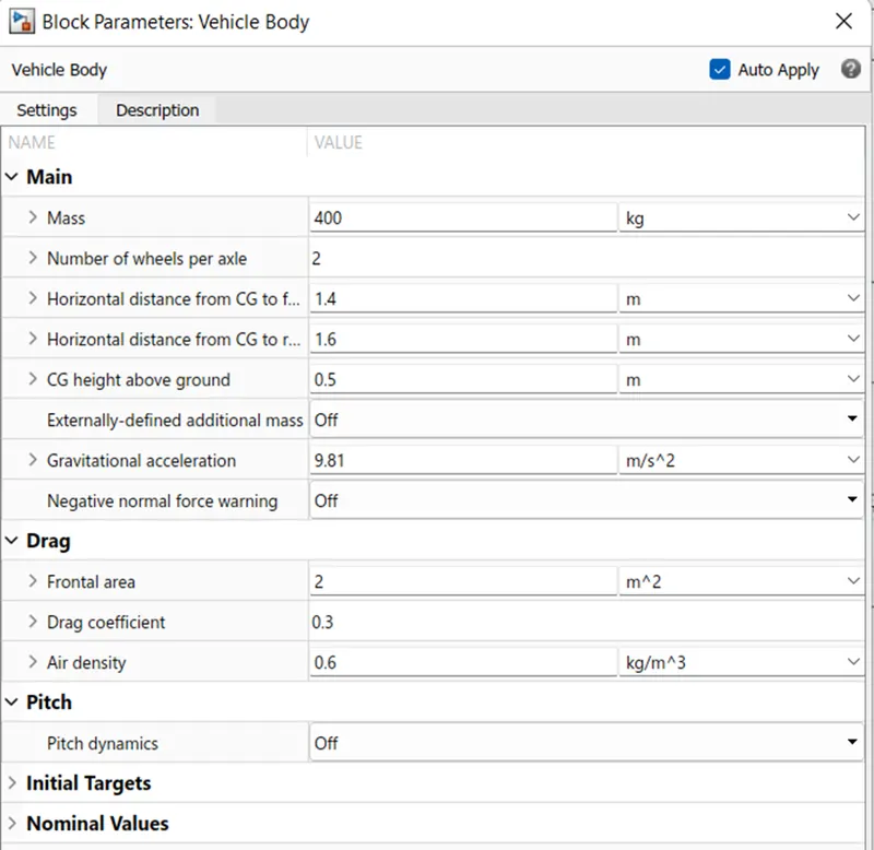
A Rear-wheel drive model of a three-wheel passenger electric rickshaw is developed. One wheel place at the front portion and the other two placed at the rear portion. The rear wheels are driven by an DC motor which is controlled by H bridge. The vehicle body designed by using three wheels with considering initial parameters of environments like wind, inclined and throttle. For simplicity grade, environmental factors are considered negligible. Before performing the modelling of the three-wheel electric vehicle drive train, we finalize the parameters and behaviour of the vehicle body. The vehicle parameters are chosen to be Settings.

Tire:

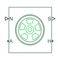
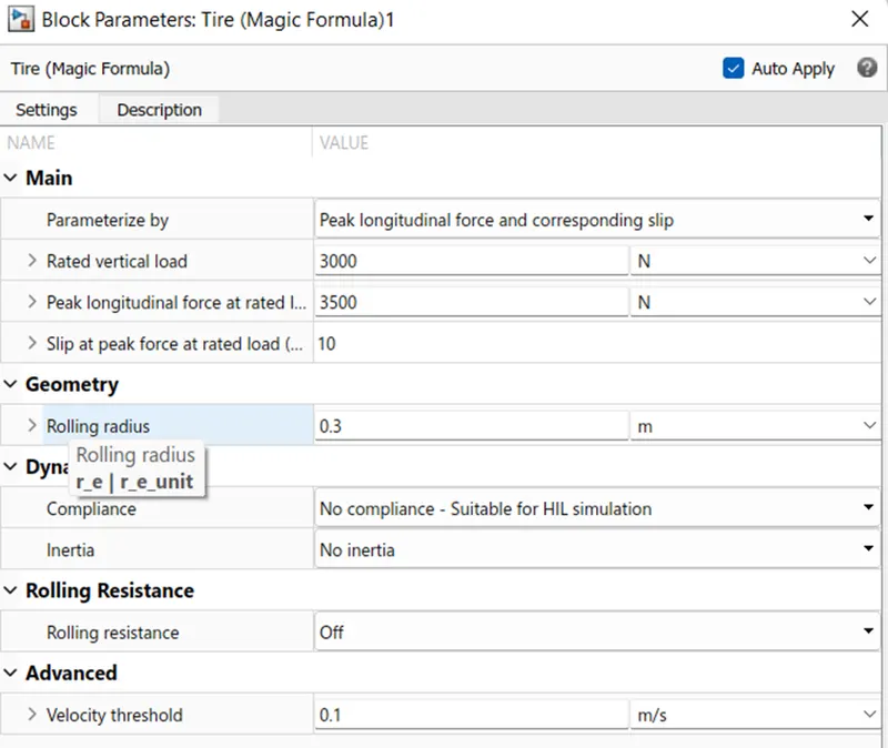
This block represents the longitudinal behaviour of a highway tire characterized by the tire magic formula. Connection A is the mechanical rotational conserving port for the wheel axle. Connection H is the mechanical translational conserving port for the wheel hub through which the thrust developed by the tire is applied to the vehicle. Connection N is the physical signal input port that applies the normal force acting on the tire. Connection S is a physical signal output port that reports the tire slip.

Drive Cycle:

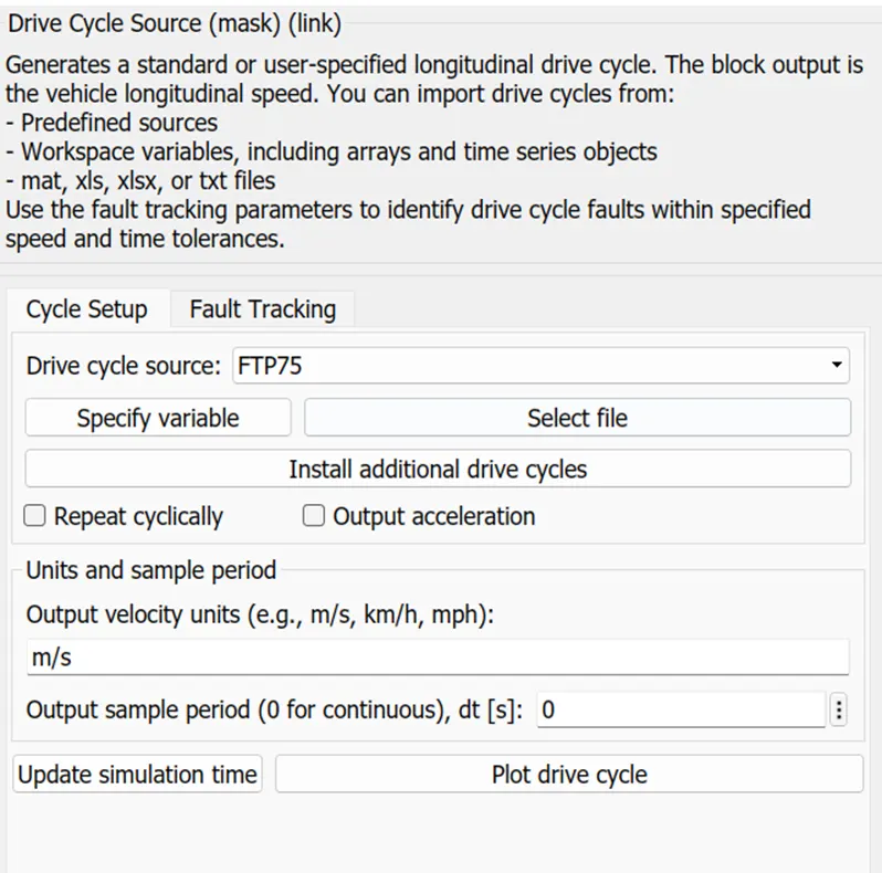
A drive cycle is typically represented by a series of data points which plots vehicle speed against time. Driving cycles are produced to assess the performance of vehicles in various ways, including fuel consumption and pollutant emissions. This is being modelled in MATLAB using drive cycle source.

Longitudinal Driver:

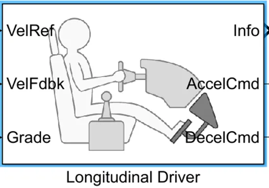
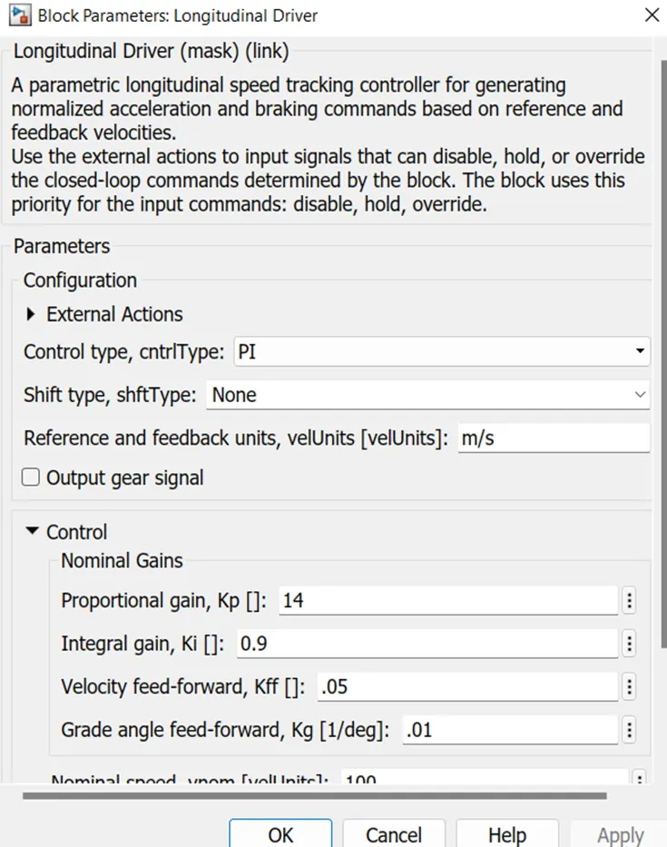
Longitudinal driver block is a parametric longitudinal speed tracking controller for generating normalized acceleration and braking commands based on reference and feedback velocities.

Longitudinal driver block includes a velocity feedback, velocity input, acceleration command and deceleration command.

Controlled PWM Voltage

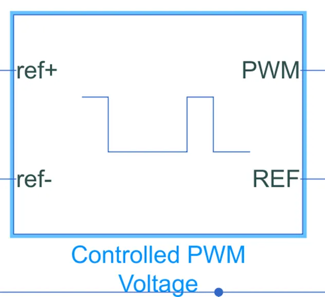
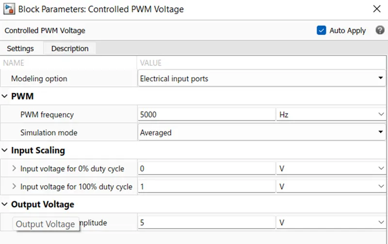
This block creates a Pulse-Width Modulated (PWM) voltage across the PWM and REF ports. The output voltage is zero when the pulse is low, and is equal to the Output voltage amplitude parameter when high. Duty cycle is set by the input value.

The Simulation mode can be set to PWM or Averaged. In PWM mode, the output is a PWM signal. In Averaged mode, the output is constant with value equal to the averaged PWM signal.

H-Bridge Circuit

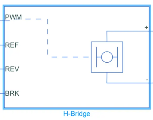
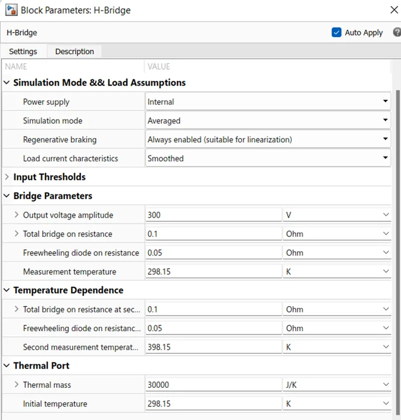
This block represents an H-bridge motor drive. The block can be driven by the Controlled PWM Voltage block in PWM or Averaged mode. In PWM mode, the motor is powered if the PWM port voltage is above the Enable threshold voltage. In Averaged mode, the PWM port voltage divided by the PWM signal amplitude parameter defines the ratio of the on-time to the PWM period. Using this ratio and assumptions about the load, the block applies an average voltage to the load that achieves the correct average load current. The Simulation mode parameter value must be the same for the Controlled PWM Voltage and H-Bridge blocks.

If the REV port voltage is greater than the Reverse threshold voltage, then the output voltage polarity is reversed. If the BRK port voltage is greater than the Braking threshold voltage, then the output terminals are short circuited via one bridge arm in series with the parallel combination of a second bridge arm and a freewheeling diode. Voltages at ports PWM, REV and BRK are defined relative to the REF port.

DC Motor

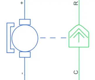
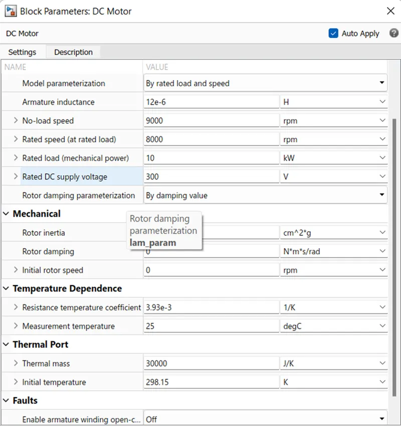
The dc motor block is used to represent the electrical and torque characteristics of the motor. Motor parameters are specified directly or derived from rated load and stall torque.

Simple Gear:

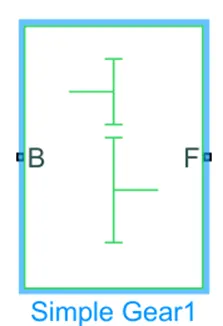
This Simple Gear Block represents an ideal nonplanetary, fixed gear ratio gear box. The gear is determined as the ratio of the input shaft angular velocity to that of the output shaft.

Battery:

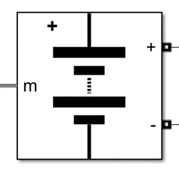
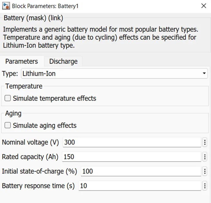
This Battery block implements a generic dynamic model that represents most popular types of rechargeable batteries. Here we used Lithium-ion type of battery.

Controlled Voltage Source:

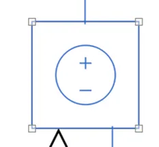
This block provides the necessary voltage that is required for the vehicle. The Controlled Voltage Source block converts a Simulink input signal into an equivalent voltage source. The generated voltage is driven by the input signal of the block. We can initialize the Controlled Voltage Source block with a specific AC or DC voltage. If we want to start the simulation in steady state, the Simulink input must be connected to a signal that begins the simulation as a sinusoidal or DC waveform that corresponds to the initial values.

Controlled Current Source:

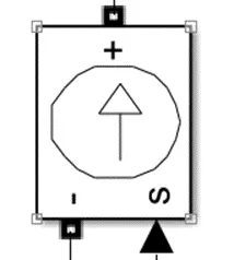
Similar to voltage block this block produces an ideal current that is powerful enough to maintain the specified current regardless of the voltage across it.

Working

In this model input signal or drive cycle data is given to longitudinal driver block. The controlled PWM signals generate PWM signals for turning ON and turning off the switches in H bridge rectifier which controls the motor circuit. Th motor gives the required torque output and velocity output can be fed back to the longitudinal driver. The speed of vehicle and output velocity of the vehicle can be compared in the scope.

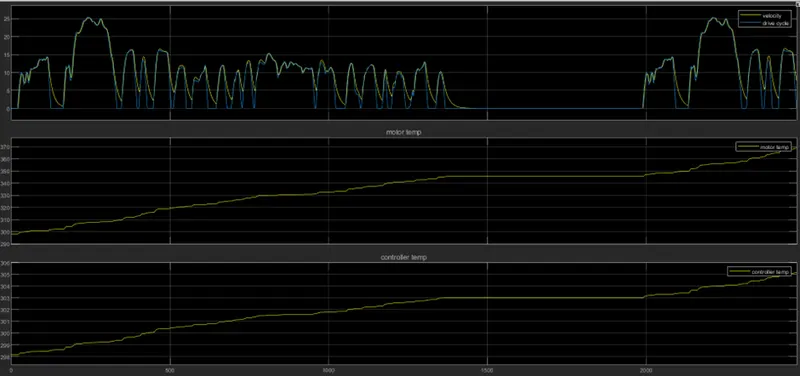
Now run the simulation using FTP75 drive cycle source for 2474 seconds and check the output results

Results of the Electric Rickshaw for FTP75 drive cycle:

Velocity, Motor temp. and Controller temp. graph:

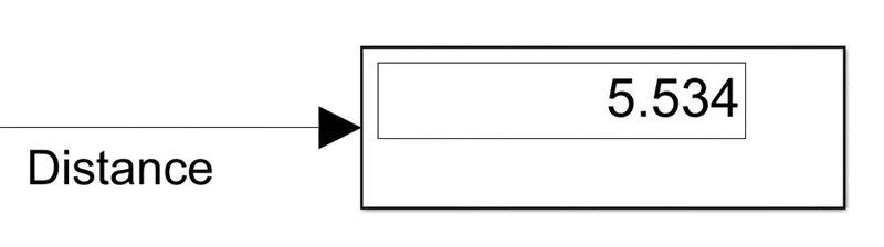
Distance travelled by vehicle:

SOC (%):

Energy Consumption:

• From the above results we can observe that the velocity of the vehicle is following the given input i.e., FTP75 drive cycle.
• The vehicle travel distance for FTP75 drive cycle for the simulation time 2474 sec. is 5.534 KM.
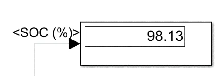
• State of the battery is 98.13%. So, we can conclude that not much discharge of the battery for FTP75 drive cycle.
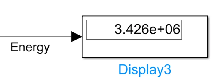
• Energy consumption is 3.4MJ.
• From the graph we also observe that temperature of the controller and motor
• I have considered initial temperature for both and controller as 298.15K and after running the simulation for 2474sec. controller temperature is increased to 305K and motor temperature increased to 370K.

Results of the Electric Rickshaw for WOT drive cycle:

Velocity, Motor temp. and Controller temp. graph:

Distance travelled by vehicle:

SOC (%):

Energy Consumption:

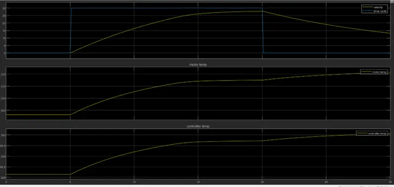
• From the above results we can observe that the velocity of the vehicle is following the given input i.e., WOT drive cycle.
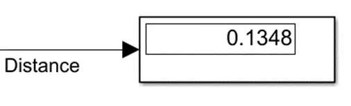
• The vehicle travel distance for WOT drive cycle for the simulation time 30 sec. is 0.134 KM.
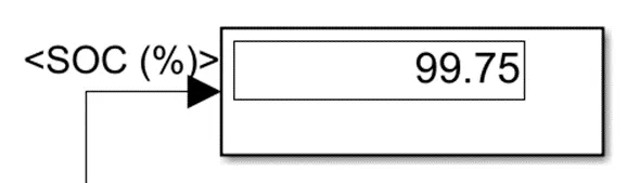
• State of the battery is 99.75%. So, we can conclude that not much discharge of the battery for WOT drive cycle.
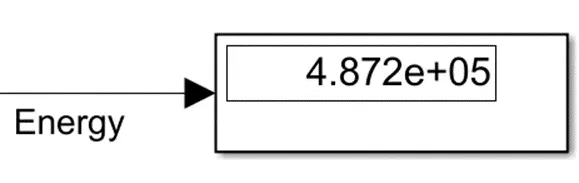
• Energy consumption is 0.48MJ.
• From the graph we also observe that temperature of the controller and motor
• I have considered initial temperature for both and controller as 298.15K and after running the simulation for 2474sec. controller temperature is increased to 301K and motor temperature increased to 315K.

Results of the Electric Rickshaw for drive cycle for 100 km constant speed driving at 45 kmph:

Velocity, Motor temp. and Controller temp. graph:

Distance travelled by vehicle:

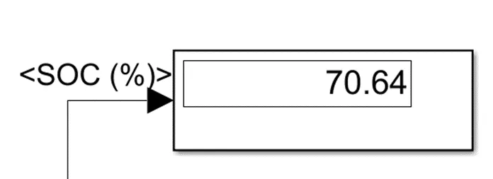
SOC (%):

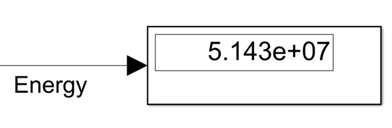
Energy Consumption:

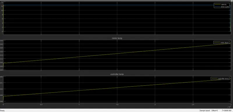
• From the above results we can observe that the velocity of the vehicle is following the given input i.e., drive cycle with 45kmph constant speed over 100km.
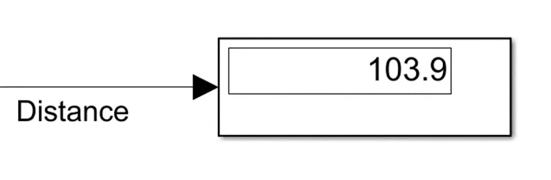
• The vehicle travel distance for given drive cycle for the simulation time 30000 sec. is 103.9 KM.
• State of the battery is 70.64%. So, we can conclude that 30% of the battery discharged for given drive cycle.
• Energy consumption is 51.48MJ. This is the highest energy consumption among the all three drive cycles.
• From the graph we also observe that temperature of the controller and motor
• I have considered initial temperature for both and controller as 298.15K and after running the simulation for 2474sec. controller temperature is increased to 302K and motor temperature increased to 333K.

Conclusion

The above electric rickshaw model has been created with all the necessary components using the SIMULINK and the model is simulated for three drive cycles. This simulation gives the vehicle speed output, current flowing from the battery, state of charge, distance travelled by vehicle, temperature rise of motor and controller and energy consumption for different drive cycles. This Electric rickshaw model covers 5.5km for FTP75 drive cycle with simulation time 2474sec., 0.13km for WOT drive cycle for simulation time 30sec, 103.9km for 45kmph constant speed drive cycle over the 100km distance for 30000sec. For FTP75 drive temperature rise more than other two drive cycles maybe its due to frequent varying of acceleration and deceleration so, frequent switching operation is required so more heat generated and energy consumption of the vehicle is high 51.4MJ for 45kmph constant speed drive cycle.