External Flow Simulation over a Cylinder
Aim: The goal of the project is to simulate the external flow on a cylinder for varying Reynolds Numbers and observe velocity and pressure profiles.
Background:
Reynold's Number: The Reynolds number is the ratio of inertial forces to viscous forces within a fluid that is subjected to relative internal movement due to different fluid velocities. A region where these forces change behavior is known as a boundary layer, such as the bounding surface in the interior of a pipe. The Reynolds number helps predict flow patterns in different fluid flow situations. At low Reynolds numbers, flows tend to be dominated by laminar flow, while at high Reynolds numbers flows tend to be turbulent.
Laminar flow is characterized by smooth streamlines and developed flow. It occurs at Reynolds numbers of 2500 and below. The layers of the fluid are parallel to each other and there is no mixing. The velocity is constant at any given moment.
Turbulent flow is characterised by fluctuations and disorderly flow. It occurs at Re 4000 and above. The streamlines of flow are irregular and layers of fluid are not parallel to each other.
Here, we will be running a base simulation at 1 m/s, and then increasing the velocity as per an increase in Reynolds number in steps of 10%. Reynolds number varies by the below formula:
Formula for Re:
`Re=((ρ*v*D))/μ`
where,
`ρ=Density ( (kg) /m^3 ) = 1000`
`v=Velocity (m/s)`
`D= Diameter (m) = 0.009`
`μ=Dynamic Viscosity (Pa.s or (N.s)⁄m^2 or kg⁄(m.s)) = 8.9 * 10^-4`
`v = (distance)/(time)`
where distance is the total length of the bounding box, and time is the flow through time we get by dividing distance by flow velocity. Total Analysis time = 2 x Flow through time
| Sl. No. | Re | %age increase over base value | Velocity (m/s) | Flow through time (s) | Total Analysis Time (s) |
| 1 | 2684.93 | 0 | 1 | 0.32 | 0.64 |
| 2 | 3221.92 | 20 | 1.2 | 0.267 | 0.534 |
| 3 | 3758.9 | 40 | 1.4 | 0.23 | 0.46 |
| 4 | 5369.86 | 100 | 2 | 0.16 | 0.32 |
Procedure:
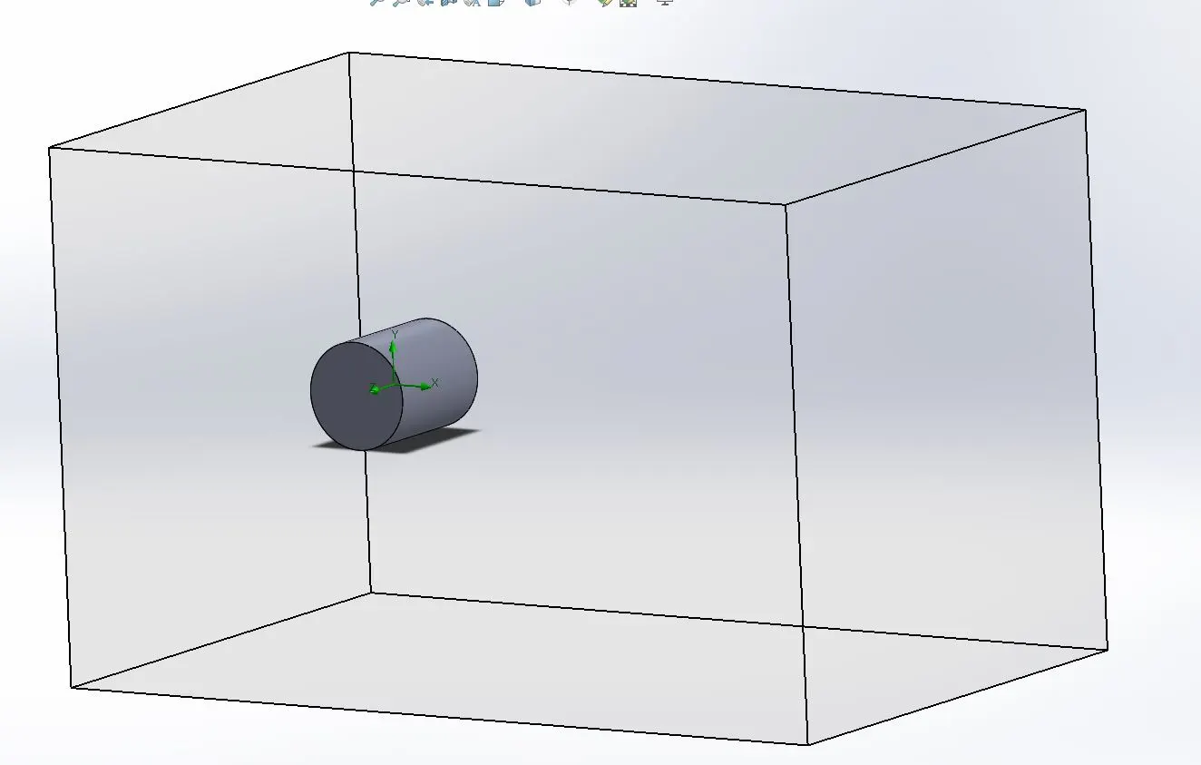
- Model a cylinder of 40 mm Diameter and 50 mm length
- Since this is an external flow, keep in mind the following bounding box dimensions
- Upstream along X= 2 times of diameter = 80 mm
- Downstream along Y = 6 times of diameter = 240 mm
- Y and Z dimensions = 100mm
- Select "External" flow in the simulation Wizard.
- Select "Time-Dependent" with the following settings (this is the base simulation):
- Total Analysis Time-> 0.64
- TIme step-> 0.01
- Select air for the fluid
- Velocity = 1 m/s
- Under Mesh, make the mesh Finer along X and Y as this is primarily a 2D simulation. Here, we have taken the following values:
- X = 50
- Y = 50
- Z = 26
- Place cut plots on XY Plane for velocity and pressure
- Run the simulation
- Finally, under animations, Create one each for Pressure and velocity cut plots.
- In the animation wizard, select "Scenario", which should show us the animation in the selected plots
Results:
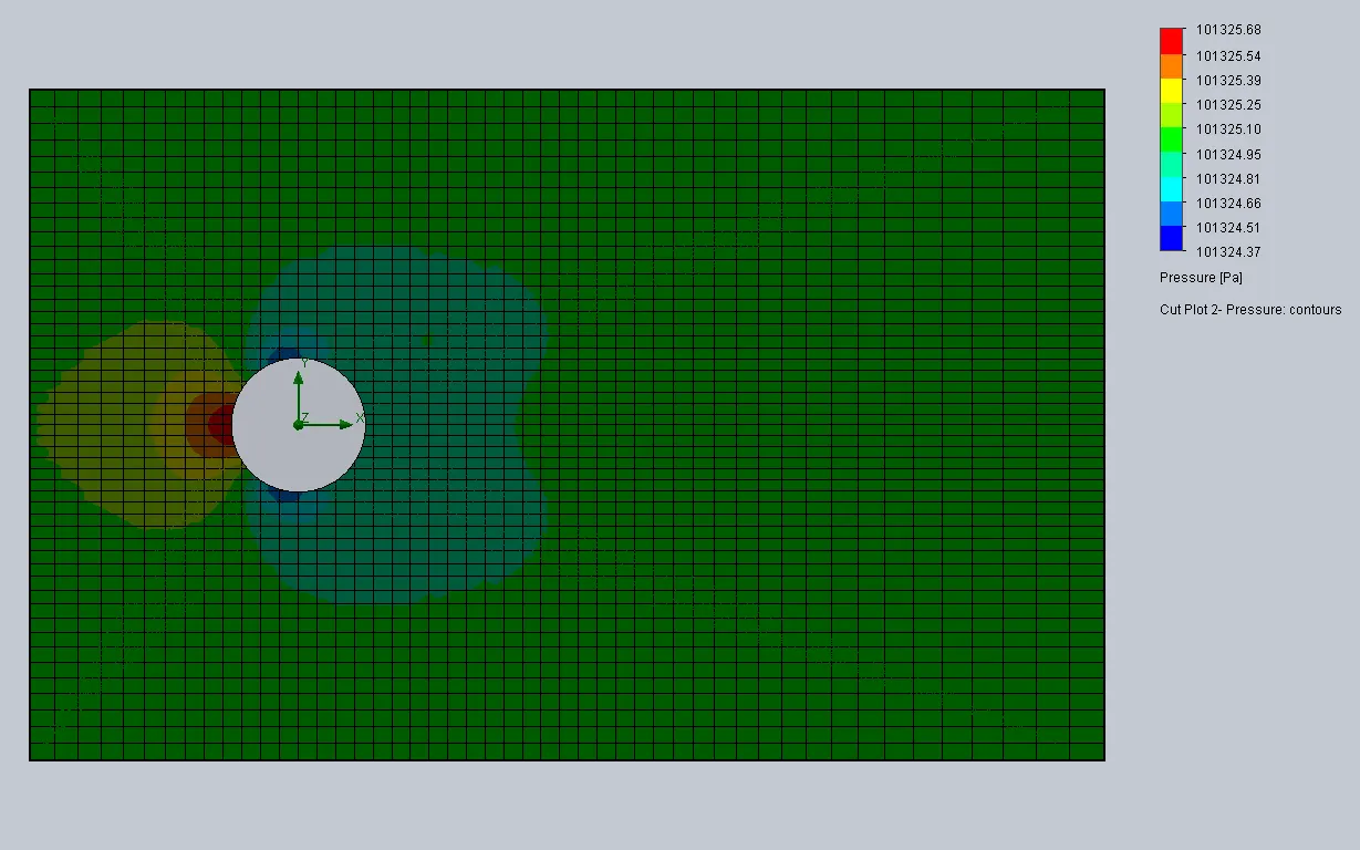
- Re = 2684.93, v = 1m/s (base):
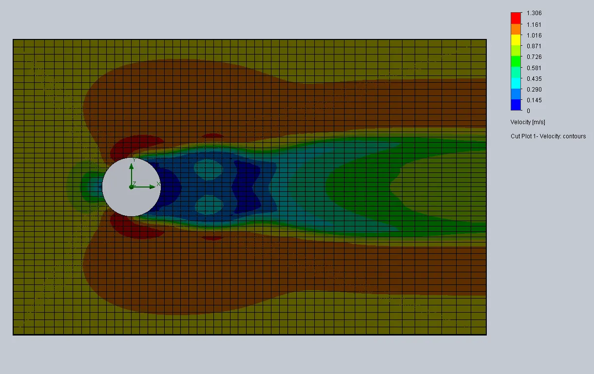
- Velocity:
- Pressure:
- Velocity:
- Re = 3221.92, v = 1.2m/s (20% increase):
- Velocity:
- Pressure:
- Velocity:
- Re = 3758.9, v = 1.4m/s (40% increase):
- Velocity:
- Pressure:
- Velocity:
- Re = 5369.86, v = 2m/s (100% increase):
- Velocity:
- Pressure:
- Velocity:
Conclusion:
Velocity plots for the baseline simulation, 40% increase and 100% increase show similar features, with only a velocity increase from 1.3 to 1.8 to 2.5 m/s respectively. These plots show unsteady-state flow.
The Velocity plot for 20% increase seems to show a highly unsteady-state flow, with flow only reaching 0.6 m/s in the wake region and about 1.18 m/s above and below the cylinder.
Pressure plots show ver little variation between all 4.