Simulation of Fluid Flow in a Pipe in Solidworks
Aim: The goal of the project is to simulate the flow in a cylindrical pipe for multiple Reynolds Number values and observe the flow development and velocity profiles for the above cases.
Background:
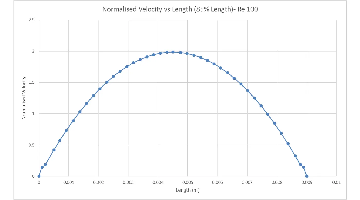
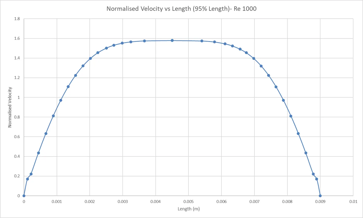
Reynold's Number: The Reynolds number is the ratio of inertial forces to viscous forces within a fluid that is subjected to relative internal movement due to different fluid velocities. A region where these forces change behavior is known as a boundary layer, such as the bounding surface in the interior of a pipe. The Reynolds number helps predict flow patterns in different fluid flow situations. At low Reynolds numbers, flows tend to be dominated by laminar flow, while at high Reynolds numbers flows tend to be turbulent.
Laminar flow is characterized by smooth streamlines and developed flow. It occurs at Reynolds numbers of 2500 and below. The layers of the fluid are parallel to each other and there is no mixing. The velocity is constant at any given moment.
Turbulent flow is characterised by fluctuations and disorderly flow. It occurs at Re 4000 and above. The streamlines of flow are irregular and layers of fluid are not parallel to each other.
In this project, we will be analysing the flow through a cylinder for 3 Reynolds numbers: 100, 1000, 10000.
Formula for Re:
`Re=((ρ*v*D))/μ`
where,
`ρ=Density ( (kg) /m^3 ) = 1000`
`v=Velocity (m/s)`
`D= Diameter (m) = 0.009`
`μ=Dynamic Viscosity (Pa.s or (N.s)⁄m^2 or kg⁄(m.s)) = 8.9 * 10^-4`
| Sl. No. | Re | Velocity (m/s) |
| 1 | 100 | 0.01113 |
| 2 | 1000 | 0.1113 |
| 3 | 10000 | 1.113 |
We will observe the differences in velocity profile and plots of velocity.
Procedure:
- Model and simulation setup:
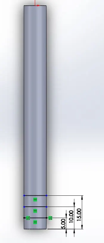
- Prepare a cylindrical shell of 10mm diameter, 0.5 mm wall thickness, and 100 mm length.
- Draw line sketches at 95%, 90% and 85% of the length from the inlet side.
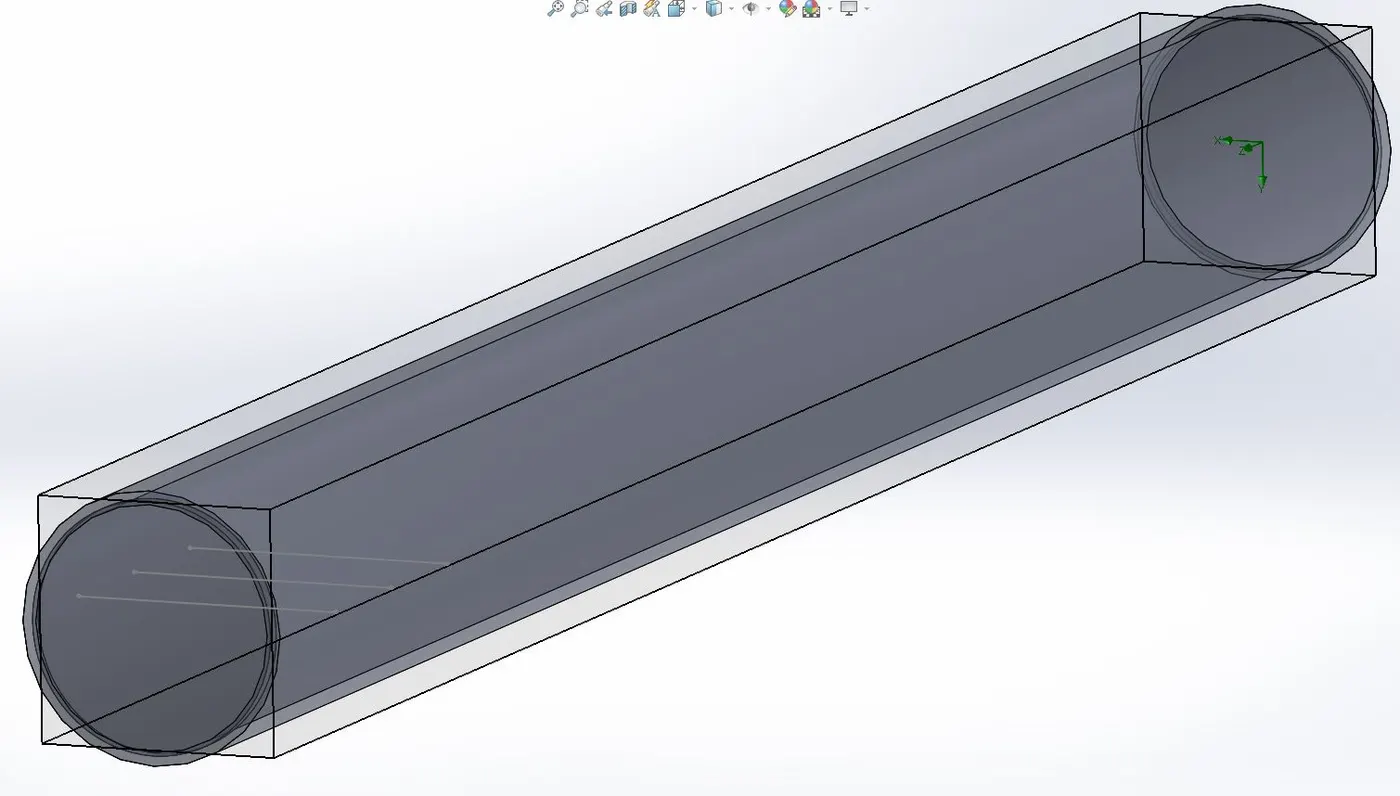
- Go to flow simulation and activate lids on the 2 faces.
- In general, settings, select water and ensure the temperature is 293 K
- Boundary Conditions:
- Inlet velocity-> as per the table shown above for 3 different cases
- Outet-> Static Pressure at NTP
- Wall-> Real wall
- Edit the number of cells per axis in the Global Mesh to 10 on x and y, 100 on z. This makes the mesh finer. (We will double these values in the parametric study)
- Run the simulation
- Parametric study setup:
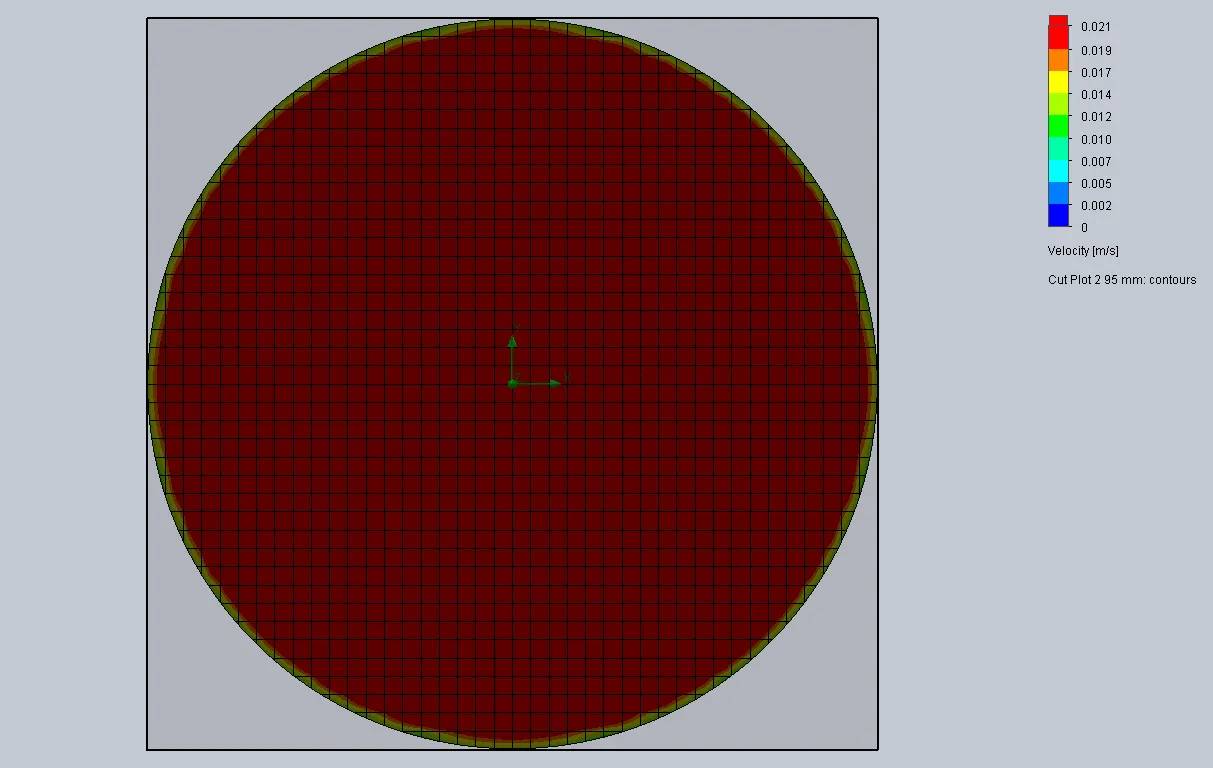
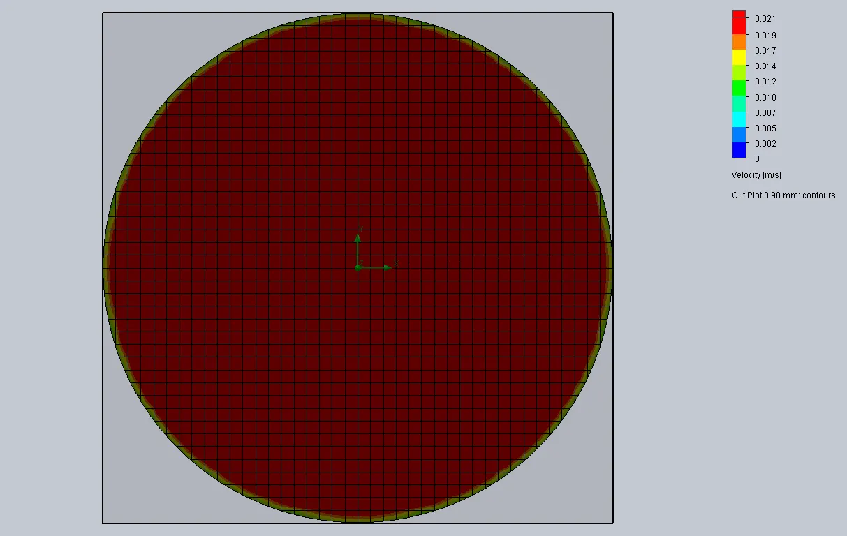
- Create cut plots at each of the probe lengths by clicking on cut plot, selecting the plane parallel to the plane where the origin is, and passing through each probe.
- Mention the contour's range as global maximum and minimum.
- Under plots, create XY plots for velocity magnitude at the 3 lengths
- Start a parametric study and add all the cut plots and XY plots as output results.
- Under Scenarios, add twice and four times the number of X, Y, and Z mesh elements for 2 new design points.
- Run the simulation and save the results. Plotting is done in excel.
Results:
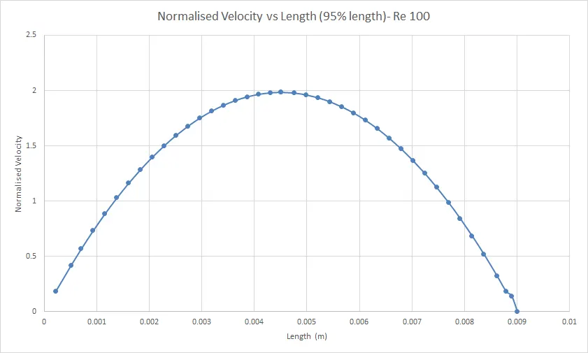
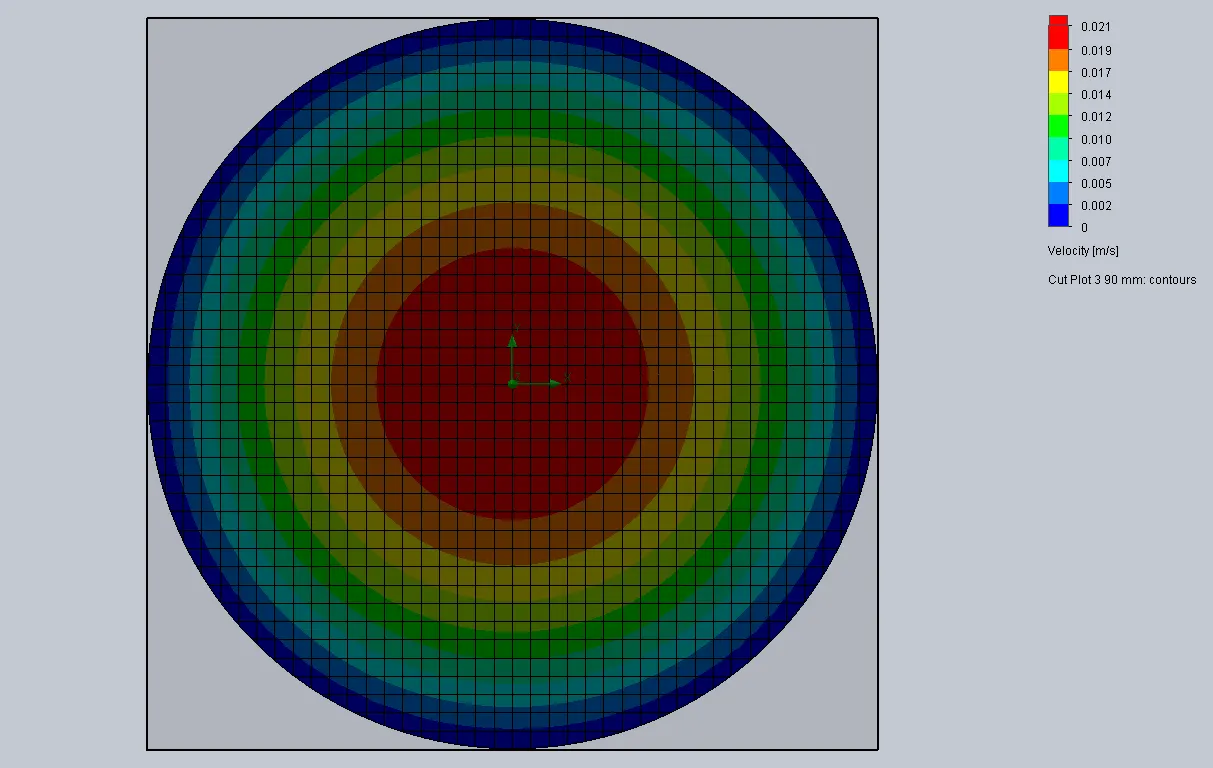
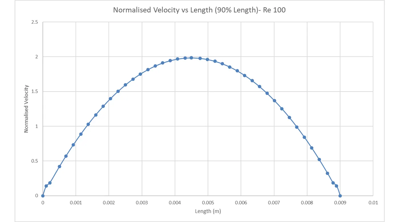
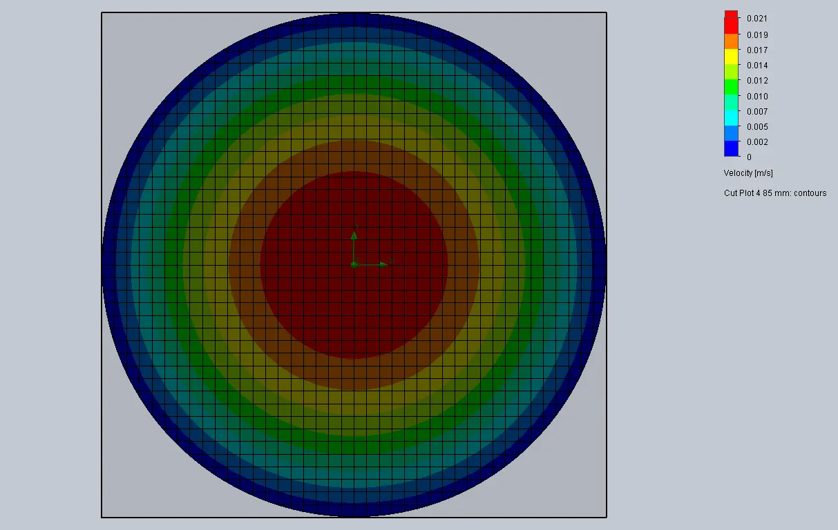
Flow at outlet, lowest number of mesh elements (10) and Re= 100:
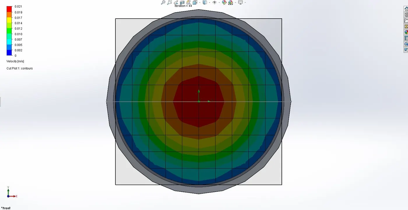
- Re 100:
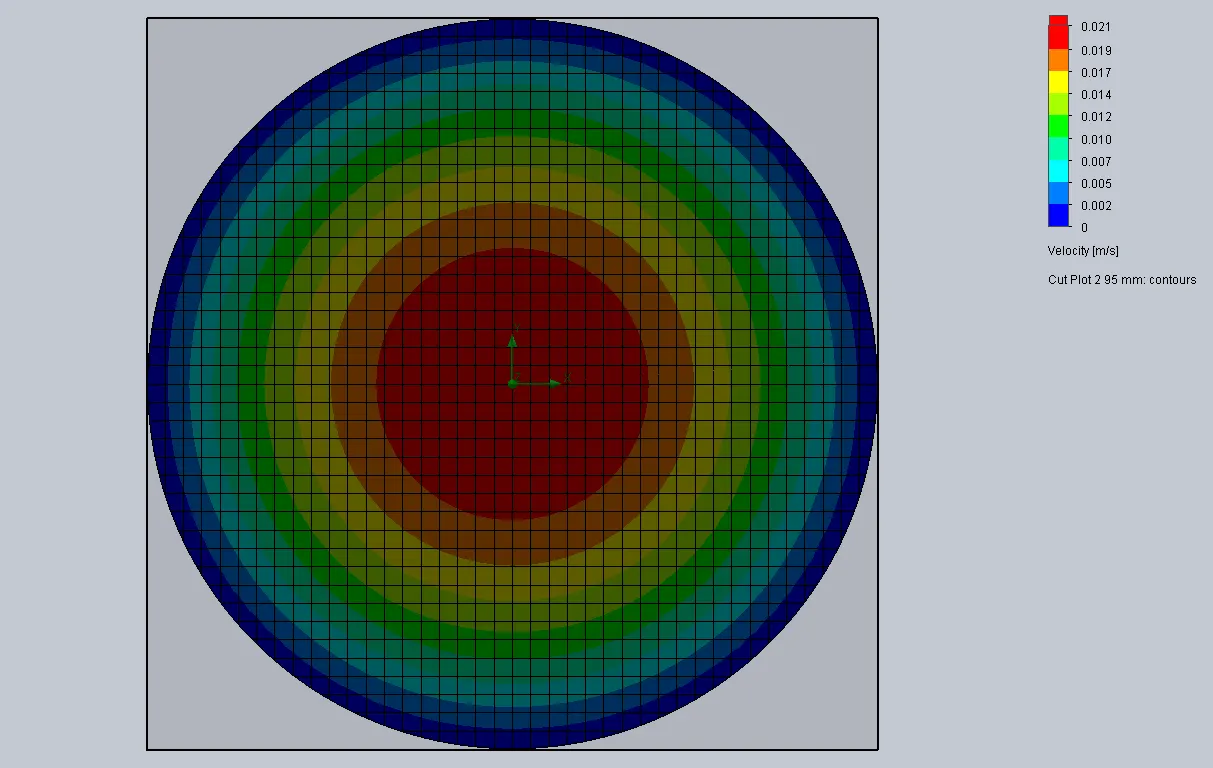
- 95% Length:
- 90% Length:
- 85% Length:
- 95% Length:
- Re 1000:
- 95% Length:
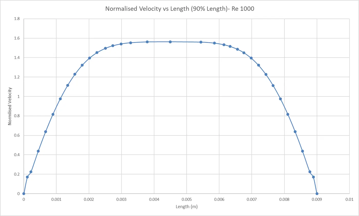
- 90% Length:
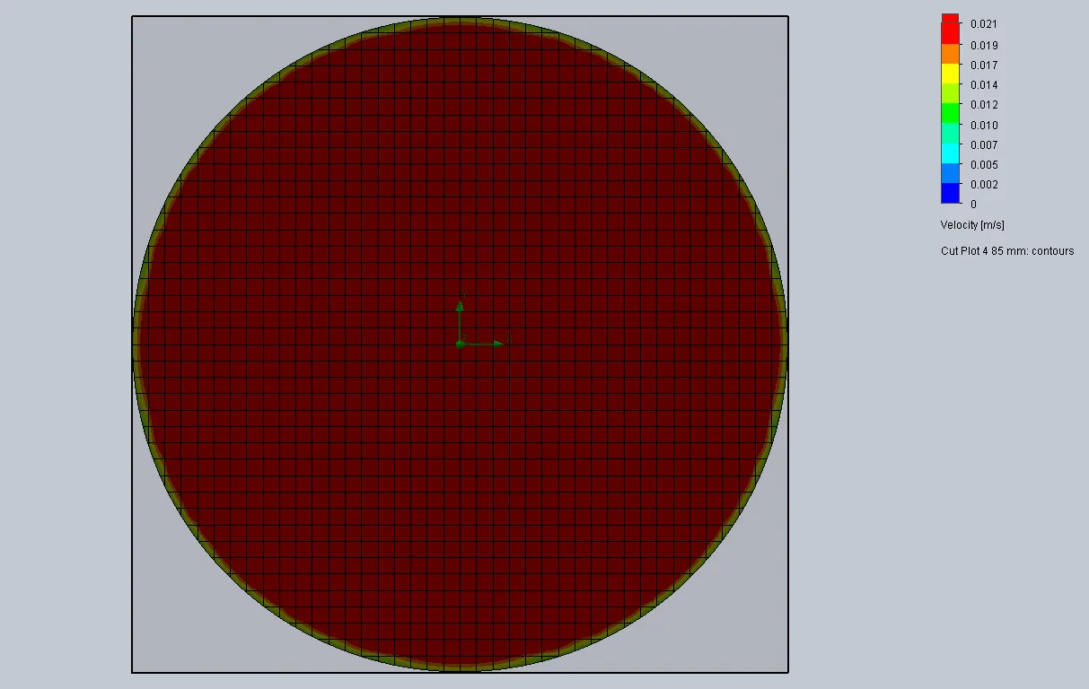
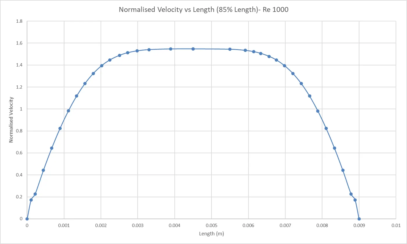
- 85% Length:
- 95% Length:
- Re 10000:
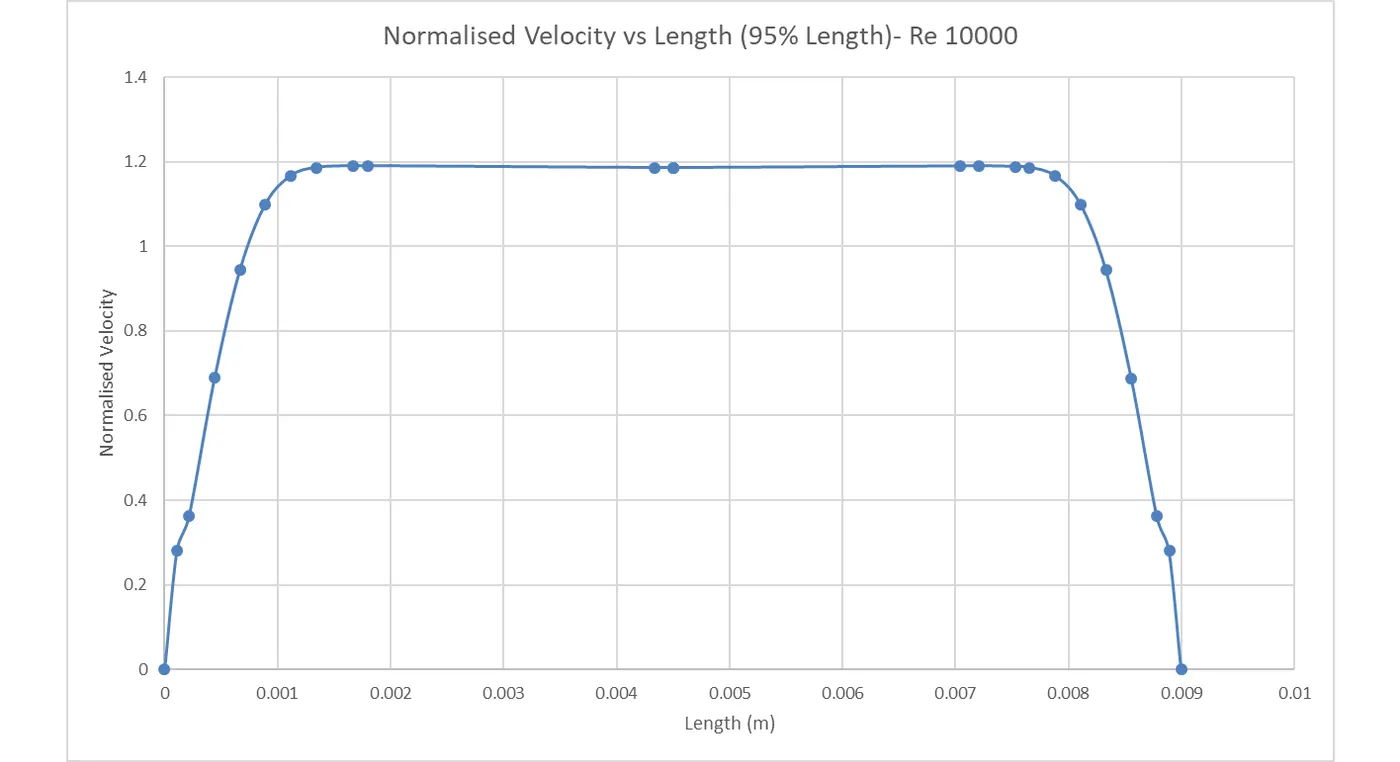
- 95% Length:
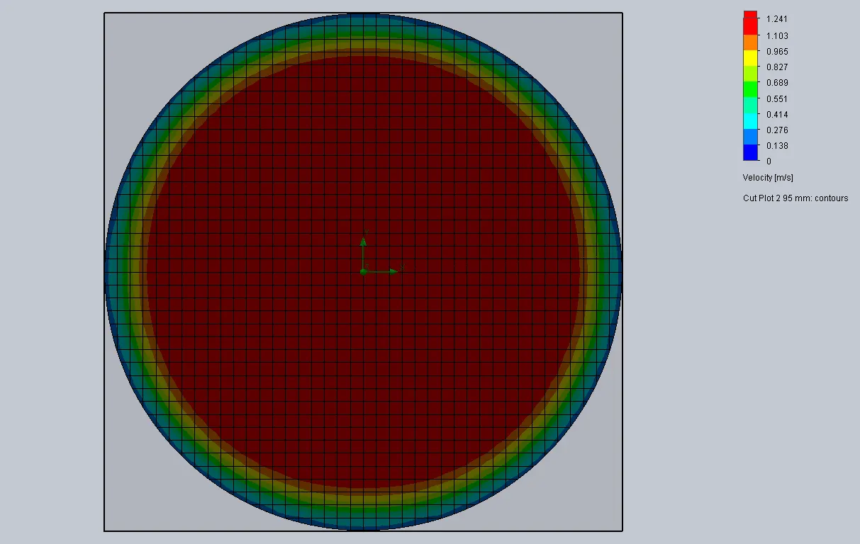
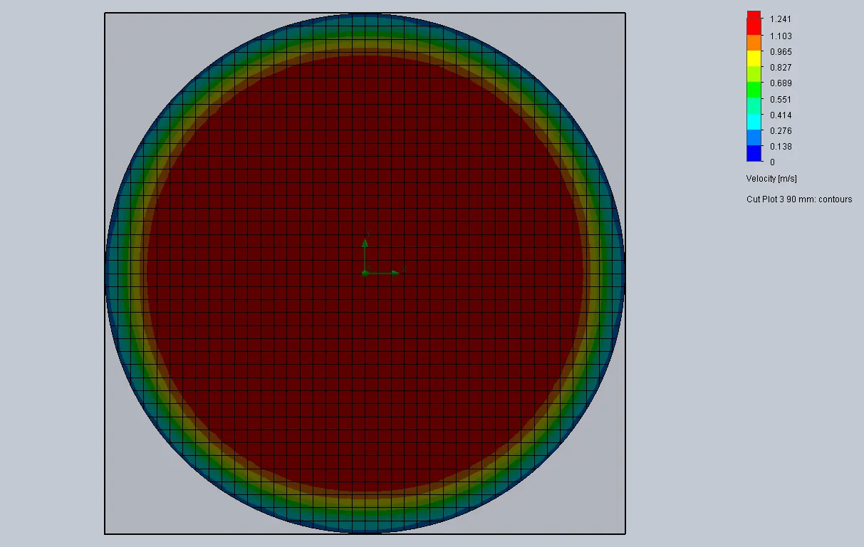
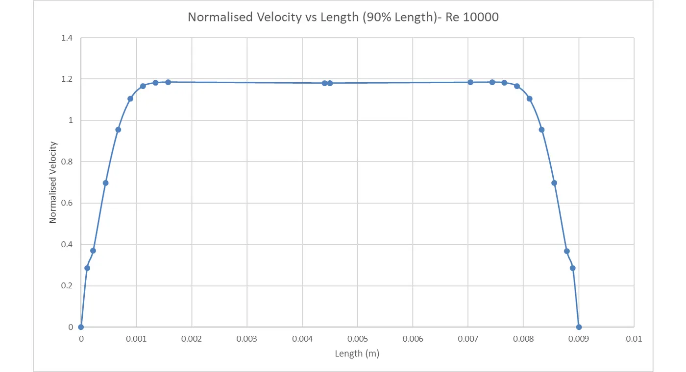
- 90% Length:
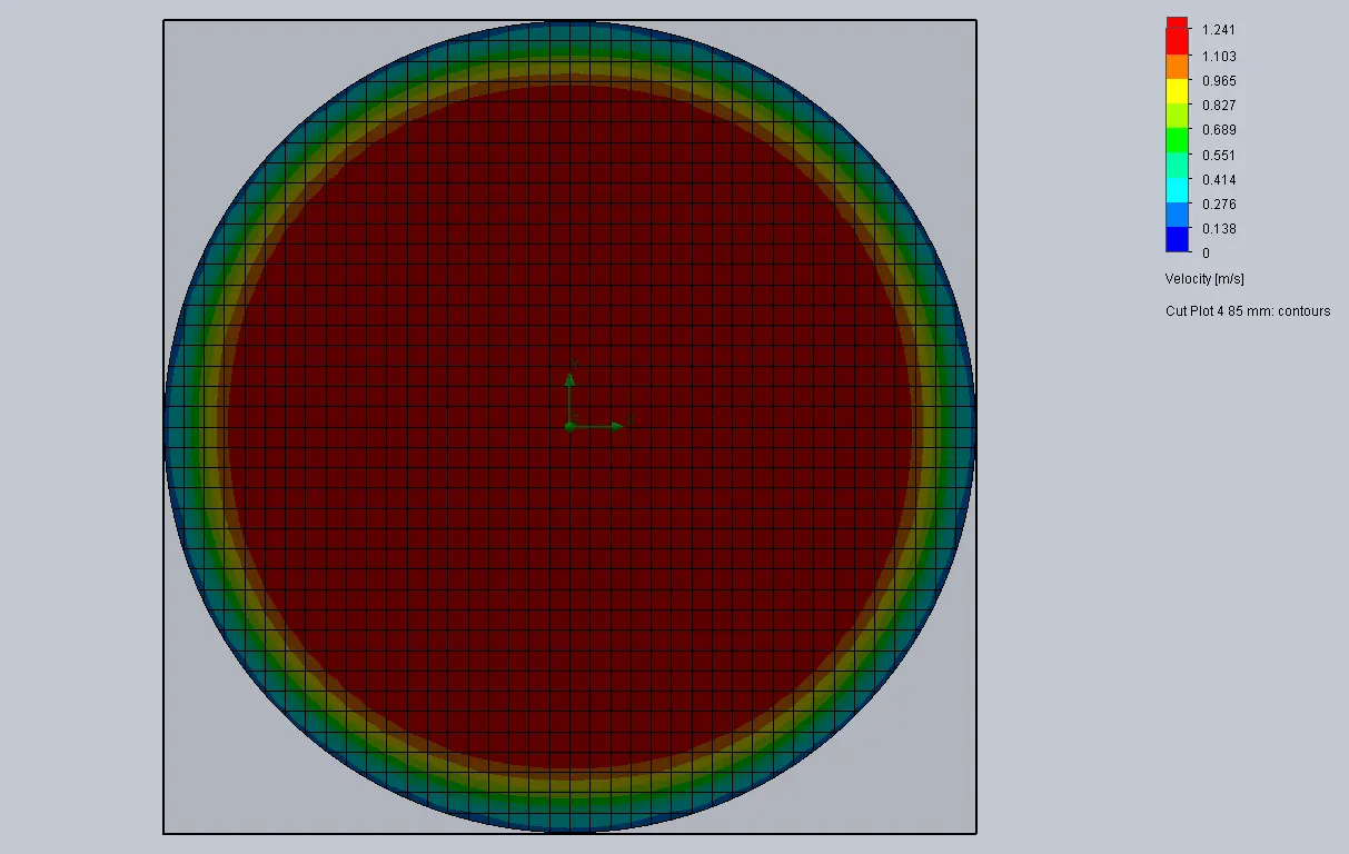
- 85% Length:
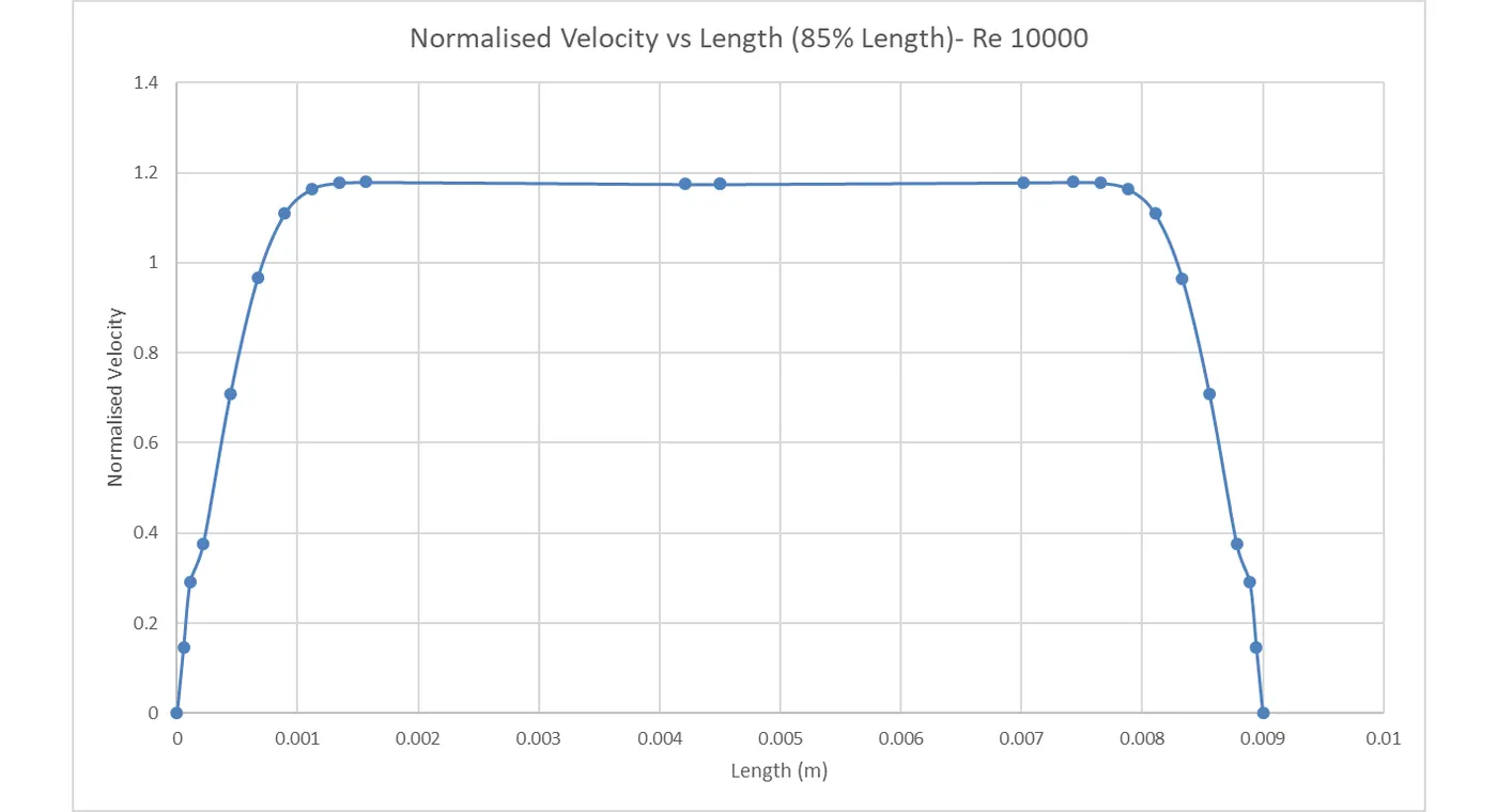
- 95% Length:
Conclusion:
Increasing Re increases velocity, which leads to flow change from Laminar to Turbulent flow. The points above show finer mesh at 4 times the original number of elements in the mesh and the results are more accurate, as seen in the difference in the cut plot from the 1st image to each of the consequent images.