Curve fitting using Python

Objective:

To find a good fitting function for showing the relationship between temperature and specific heat capacity at constant pressure using the practical values from the data file

Procedure:

• First, we define a function f(x) which will be will give the relationship between the temperature (x) and Cp (y) values
• Then, a function is defined which will read and arrange the contents of the data file
• In the main program, we use the curvefit function from the scipy module to calculate the coefficients of x in f(x)
• Then, we after f(x) is defined fully, we use it to calculate the theoritical values of y
• And then, plot the curve between the actual data points and the points we get from the calculated f(x)
• And finally, we have used the `R^2`method from statistics to calculate the goodness of fit.

where, `R^2` lies between 0 and 1. The closer its value is to 1, the better is the fit.

Here, `R^2= (SSR)/(SST)`

SSR = Sum of squares of regression or amount of variance captured by the function

SST = Sum of squares of total or amount of variance in data

Case 1: Taking f(x) as a linear equation

Code:

import math
import matplotlib.pyplot as plt
import numpy as np
from scipy.optimize import curve_fit

#define a function which will act as the fitting curve for the data points 
def func(t,a,b):
	return a*pow(t,1)+b

#function to read the data from data file
def readfile():
	temperature=[]
	cp=[]
	for line in open('data','r'):
		values=line.split(',')
		temperature.append(float(values[0]))
		cp.append(float(values[1]))

	return (temperature,cp)
	
#calling the function to read the data from the file store them in the following variables	
temperature,cp=readfile()

#invoking the curvefit function to get the values of coefficients
popt,pcov=curve_fit(func,temperature,cp)

#calculating the values of Cp from the function
fit_cp=func(np.array(temperature),*popt)

#plotting the actual curve against the curve given by the function
plt.plot(temperature,cp,'r',label='Actual')
plt.plot(temperature,fit_cp,'b',label='Calculated')
plt.title('Comparision of actual vs calculated curve')
plt.xlabel('Temperature')
plt.ylabel('Specific heat capacity at constant pressure')
plt.legend(loc='best')	
plt.show()	

#checking for goodness of fit with R^2 calculation

#mean of actual cp values 
mean_cp=sum(cp)/len(cp)

#Sum of squares of total or amount of variance in data
SST=sum(pow((np.array(cp)-mean_cp),2))

#Sum of squares of regression or amount of variance captured by the function
SSR=sum(pow((np.array(fit_cp)-mean_cp),2))

#R^2=SSR/SST
print('R Square:',SSR/SST)

Results:

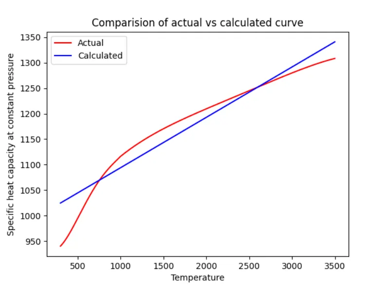
Here, the curve seems to be not fitting very well with the actual values. Also, the value of `R^2`comes out to be ~0.92 and hence it has lot of scope for optimisation.

Case 2: Taking f(x) as a quadratic equation

Code:

import math
import matplotlib.pyplot as plt
import numpy as np
from scipy.optimize import curve_fit

#define a function which will act as the fitting curve for the data points 
def func(t,a,b,c):
	return a*pow(t,2)+b*pow(t,1)+c

#function to read the data from data file
def readfile():
	temperature=[]
	cp=[]
	for line in open('data','r'):
		values=line.split(',')
		temperature.append(float(values[0]))
		cp.append(float(values[1]))

	return (temperature,cp)
	
#calling the function to read the data from the file store them in the following variables	
temperature,cp=readfile()

#invoking the curvefit function to get the values of coefficients
popt,pcov=curve_fit(func,temperature,cp)

#calculating the values of Cp from the function
fit_cp=func(np.array(temperature),*popt)

#plotting the actual curve against the curve given by the function
plt.plot(temperature,cp,'r',label='Actual')
plt.plot(temperature,fit_cp,'b',label='Calculated')
plt.title('Comparision of actual vs calculated curve')
plt.xlabel('Temperature')
plt.ylabel('Specific heat capacity at constant pressure')
plt.legend(loc='best')	
plt.show()	

#checking for goodness of fit with R^2 calculation

#mean of actual cp values 
mean_cp=sum(cp)/len(cp)

#Sum of squares of total or amount of variance in data
SST=sum(pow((np.array(cp)-mean_cp),2))

#Sum of squares of regression or amount of variance captured by the function
SSR=sum(pow((np.array(fit_cp)-mean_cp),2))

#R^2=SSR/SST
print('R Square:',SSR/SST)

Results:

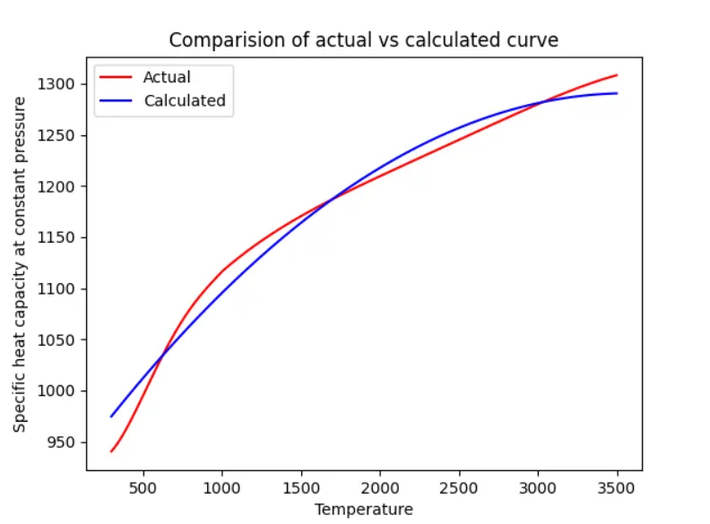
Here too, the curve seems to be not fitting very well with the actual values. Also, the value of `R^2`comes out to be ~0.98 and hence it has still a scope for optimisation.

Case 3: Taking f(x) as a cubic equation

Code:

import math
import matplotlib.pyplot as plt
import numpy as np
from scipy.optimize import curve_fit

#define a function which will act as the fitting curve for the data points 
def func(t,a,b,c,d):
	return a*pow(t,3)+b*pow(t,2)+c*pow(t,1)+d

#function to read the data from data file
def readfile():
	temperature=[]
	cp=[]
	for line in open('data','r'):
		values=line.split(',')
		temperature.append(float(values[0]))
		cp.append(float(values[1]))

	return (temperature,cp)
	
#calling the function to read the data from the file store them in the following variables	
temperature,cp=readfile()

#invoking the curvefit function to get the values of coefficients
popt,pcov=curve_fit(func,temperature,cp)

#calculating the values of Cp from the function
fit_cp=func(np.array(temperature),*popt)

#plotting the actual curve against the curve given by the function
plt.plot(temperature,cp,'r',label='Actual')
plt.plot(temperature,fit_cp,'b',label='Calculated')
plt.title('Comparision of actual vs calculated curve')
plt.xlabel('Temperature')
plt.ylabel('Specific heat capacity at constant pressure')
plt.legend(loc='best')	
plt.show()	

#checking for goodness of fit with R^2 calculation

#mean of actual cp values 
mean_cp=sum(cp)/len(cp)

#Sum of squares of total or amount of variance in data
SST=sum(pow((np.array(cp)-mean_cp),2))

#Sum of squares of regression or amount of variance captured by the function
SSR=sum(pow((np.array(fit_cp)-mean_cp),2))

#R^2=SSR/SST
print('R Square:',SSR/SST)

Results:

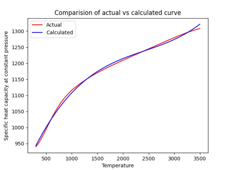
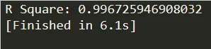
Here, the curve seems to be fitting with the actual values to a great extent. Also, the value of `R^2`comes out to be 0.9967 which is very much closer to 1 now. And hence, the result seems to be optimised.

Discussions:

As seen from the three cases, the curve fit seems to be much more optimised as the degree of polynomial is increased.

Also, here are some Q&As regarding the project:

1. What does popt and pcov mean?

Ans: popt stores the values of coefficients of x of f(x) defined above and pcov stores the estimated co-variance of popt. Its diagonals gives the variance of the parameter estimate

2. What does np.array(temperature) do?

Ans: Originally, temperature is in the form of a list and to be used in the func function, it needs to be in the array format and hence this command converts it into an array.

3. What does the * in *popt mean?

Ans: It points to the address of the coefficients stored inside popt

4. What needs to be done in order to make the curve fit perfect?

Ans: From the results, it can be seen that increasing the order of the polynomial increases the perfection of the curve.