Basics of ML & AL Week 2 Challenge

1)

The values from the table:

$$\begin{array}{rl}{\displaystyle X}& {\displaystyle :0,1,2,3,4}\\ {\displaystyle P(X)}& {\displaystyle :0.35,0.25,0.15,0.15,0.10}\end{array}$$

---

1. Mean ($\mu$):

The mean is calculated as:

$$\mu =\sum X\cdot P(X)$$$$\mu =(0\cdot 0.35)+(1\cdot 0.25)+(2\cdot 0.15)+(3\cdot 0.15)+(4\cdot 0.10)$$$$\mu =0+0.25+0.30+0.45+0.40=1.40$$

Mean ($\mu$) = 1.40

---

2. Variance (${\sigma }^2$):

The variance is:

$${\sigma }^2=\sum P(X)\cdot (X-\mu {)}^2$$

First, calculate $(X-\mu {)}^2$ for each $X$:

$$X=0(0-1.4{)}^2=1.96$$$$X=1(1-1.4{)}^2=0.16$$$$X=2(2-1.4{)}^2=0.36$$$$X=3(3-1.4{)}^2=2.56$$$$X=4(4-1.4{)}^2=6.76$$

Now calculate ${\sigma }^2$:

$${\sigma }^2=(0.35\cdot 1.96)+(0.25\cdot 0.16)+(0.15\cdot 0.36)+(0.15\cdot 2.56)+(0.10\cdot 6.76)$$$${\sigma }^2=0.686+0.04+0.054+0.384+0.676=1.84$$

Variance (${\sigma }^2$) = 1.84

---

3. Skewness:

Skewness measures the asymmetry of the distribution and is calculated as:

$$\text{Skewness}=\frac{\sum P(X)\cdot (X-\mu {)}^3}{{\sigma }^3}$$

First, calculate $(X-\mu {)}^3$ for each $X$:

$$X=0(0-1.4{)}^3=-2.744$$$$X=1(1-1.4{)}^3=-0.064$$$$X=2(2-1.4{)}^3=0.216$$$$X=3(3-1.4{)}^3=4.096$$$$X=4(4-1.4{)}^3=17.576$$

Now calculate the numerator:

$$\sum P(X)\cdot (X-\mu {)}^3=(0.35\cdot -2.744)+(0.25\cdot -0.064)+(0.15\cdot 0.216)<br>+(0.15\cdot 4.096)+(0.10\cdot 17.576)$$$$\text{Numerator}=-0.9604-0.016+0.0324+0.6144+1.7576=1.428$$

Now divide by ${\sigma }^3=(1.84{)}^{3\mathrm{<br>}}$

$${\sigma }^3=2.49$$$$\text{Skewness}=\frac{1.428}{2.49}=0.573$$

Skewness = 0.573

---

4. Kurtosis:

Kurtosis measures the "tailedness" of the distribution and is calculated as:

$$\text{Kurtosis}=\frac{\sum P(X)\cdot (X-\mu {)}^4}{{\sigma }^4}$$

First, calculate $(X-\mu {)}^4$ for each $X$:

$$X=0(0-1.4{)}^4=3.8416$$$$X=1(1-1.4{)}^4=0.0256$$$$X=2(2-1.4{)}^4=0.1296$$$$X=3(3-1.4{)}^4=6.5536$$$$X=4(4-1.4{)}^4=44.6976$$

Now calculate the numerator:

$$\sum P(X)\cdot (X-\mu {)}^4=(0.35\cdot 3.8416)+(0.25\cdot 0.0256)+(0.15\cdot 0.1296)+(0.15\cdot 6.5536)+(0.10\cdot 44.6976)$$$$\text{Numerator}=1.34456+0.0064+0.01944+0.98304+4.46976=6.822$$

Now divide by ${\sigma }^4=(1.84{)}^2=3.3856$:

$$\text{Kurtosis}=\frac{6.822}{3.3856}=2.015\mathrm{-3=-0.98}$$

The subtraction of 3 is to adjust for excess kurtosis, which compares the distribution to a normal distribution (whose kurtosis is 3).

Kurtosis = -0.98

This negative kurtosis indicates the distribution is platykurtic (flatter than a normal distribution).

---

Final Results:

1. Mean ($\mu$) = 1.40
2. Variance (${\sigma }^2$) = 1.84
3. Skewness = 0.573
4. Kurtosis = -0.98

2) What is the significance of expected value when simple mean (Sum of all observations/number of observations) is already in place?

- Expected Value:

- Used in probability distributions.

- Represents the long-term average or theoretical center of a random variable.

- Formula: E(X) = Sum(X * P(X)) (weighted average of outcomes, where weights are probabilities).

- Useful for theoretical models and predicting future outcomes based on probabilities.

- Simple Mean:

- Used for raw data.

- Formula: Mean = Sum of all observations / Number of observations.

- Assumes all observations are equally likely (no weights).

- Key Difference:

Expected value incorporates probabilities (weights), while the simple mean is an arithmetic average of observed data.

3) Having skewness in the curve considered to be bad in the analysis?

Skewness measures the asymmetry of a distribution:

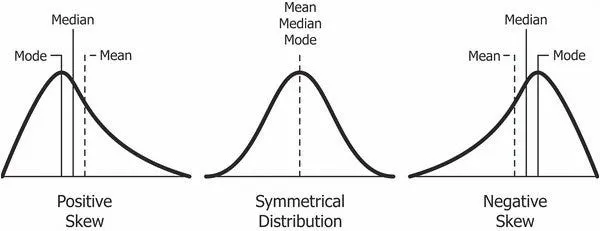
- Positive Skew: Tail is longer on the right (e.g., income data).

- Negative Skew: Tail is longer on the left (e.g., exam scores).

- No Skew: Symmetric distribution (e.g., normal distribution).

- Impact of Skewness:

- Not inherently bad: Skewness depends on the context.

- When problematic:

- If the analysis assumes normal distribution (e.g., hypothesis testing), skewness can bias results.

- Skewed data can distort measures like the mean.

- When useful:

- Skewness can highlight important insights (e.g., risks in finance, extreme values in data).

4) Evaluate probabilities for continuous normal distribution with given mean = 680 and standard deviation = 31:

z = (X – μ) / σ

a) P(X < 711)

Z = (711 - 680) / 31 = 1

Z-table: P(Z < 1) = 0.8413.

Therefore, P(X < 711) = 0.8413.

b) P(X > 740)

Z = (740 - 680) / 31 = 1.94

Z-table: P(Z > 1.94) = 1 - P(Z < 1.94) = 1 - 0.9738 = 0.0262.

Therefore, P(X > 740) = 0.0262.

c) P(600 < X < 720)

Z for 600 = (600 - 680) / 31 = -2.58

Z for 720 = (720 - 680) / 31 = 1.29

Z-table: P(Z < 1.29) = 0.9015, P(Z < -2.58) = 0.0049.

Therefore, P(600 < X < 720) = 0.9015 - 0.0049 = 0.8966.

d) P(X = 720)

For a continuous normal distribution, the probability of a single value is always 0.

For a continuous normal distribution, the probability of a random variable XXX being equal to a specific value (e.g., P(X=720)P(X = 720)P(X=720)) is always 0.

• In a continuous distribution, probabilities are calculated over intervals, not at single points.
• The area under the curve for a single point is infinitesimally small, effectively zero.
• Mathematically: P(X=c)=0P(X = c) = 0P(X=c)=0, where ccc is any specific value for a continuous random variable.

5)

The curve shown is a normal distribution curve (also known as a bell curve), which represents the distribution of data where most values cluster around the mean, and the probabilities taper off symmetrically as you move further away from the mean.

Key Features of the Curve:

1. Mean (μ):
• The center of the curve represents the mean, which is also the peak of the curve.
• It is the most common value in the dataset.
2. Standard Deviation (σ):
• The horizontal axis is marked in units of standard deviation (σ) from the mean.
• The standard deviation measures the spread of the data:
• Smaller σ: Narrower and taller curve (data is tightly clustered around the mean).
• Larger σ: Wider and shorter curve (data is more spread out).
3. Symmetry:
• The curve is perfectly symmetric about the mean.
• The left side mirrors the right side.
4. Empirical Rule (68-95-99.7 Rule):
• Approximately:
• 68% of the data falls within 1σ of the mean (μ±1σ\mu \pm 1\sigmaμ±1σ).
• 95% of the data falls within 2σ of the mean (μ±2σ\mu \pm 2\sigmaμ±2σ).
• 99.7% of the data falls within 3σ of the mean (μ±3σ\mu \pm 3\sigmaμ±3σ).

Right Side of the Curve:

• The right side of the curve corresponds to values greater than the mean.
• Probabilities decrease as you move further to the right.
• For example:
• 1σ to 2σ: About 13.6% of the data lies in this region.
• 2σ to 3σ: About 2.1% of the data lies in this region.
• Beyond 3σ: About 0.1% of the data lies here, representing extreme values (outliers).

Applications:

• This curve is used in various fields, such as statistics, finance, and science, to model real-world phenomena like test scores, heights, or measurement errors.