Assignment 3-2D Element Formulation Challenge

The goal of this assignment is to compare the results of the simulation of a beam against a rigid wall with two different 2D element formulations.

Base Simulation

Step 1: Loading the model

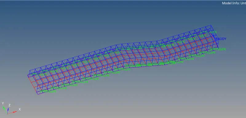
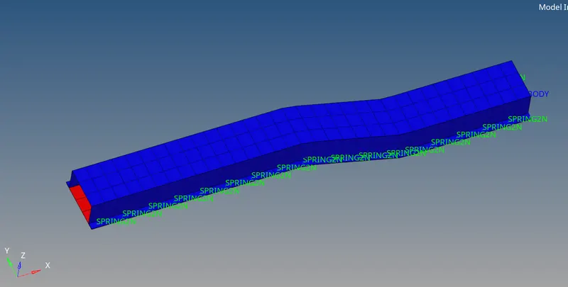
The base file is loaded into Hypermesh and the model can be observed as shown below.

Step 2: Modification of run time and plot frequency

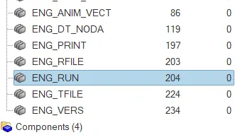
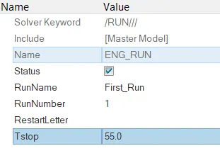
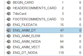
The run-time can be changed from 60 to 55ms by altering the value of Tstop in the ENG_RUN control card.

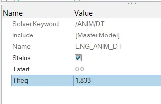
The output time step has been chosen to give 30 animation steps. Therefore the frequency Tfreq = 55/30 = 1.833.

This parameter can be adjusted in the ENG_ANIM_DT control card.

Step 3: Running the simulation

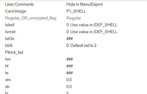
The simulation with the base element formulation parameters can be run using radioss. The default shell parameters are shown below.

• The base simulation is run without any modification to element properties using Radioss option under analysis tab.
• Create a folder to save the rad files in local directory.

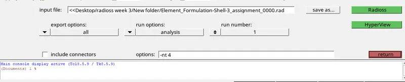
• Edit options providing number of thread as "-nt 4".
• After the simulation is run, the results can be viewed in Hyperview and Hypergraph 2D.

Step 4: Results

The total energy and the mass error can be visualized from the 0001.out file at the end of the simulation.

The acceptable error limits are:

Energy error: -15% to +5%

Mass error: upto 2

• After analysis the .OUT file is viewd to check whether the Energy Error and mass error fall within the acceptable range.

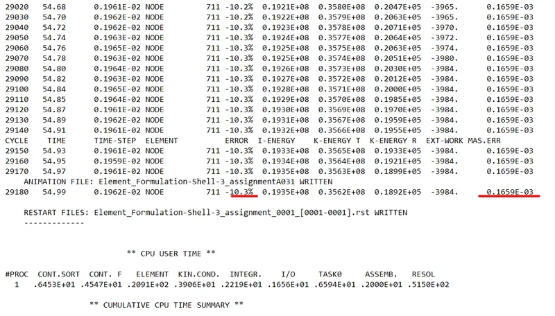
• The energy error is -10.3% and the mass error stays constant through out the simulation i.e 0.1659 e-3, both of which are within acceptable limits.
• Since the error values are acceptable,rigid wall forces,internal energy,hourglass energy,contact energy ,total energy of the simulation are plotted with the help of HYPERGRAPH 2-D.
• HYPERVIEW is opened to view the simulation .
• Model and Results(h3d file) are loaded from the newly created folder.

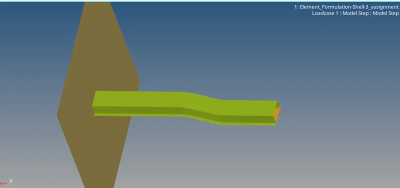
• Animations shows how the crash tube deforms under the action of force.
• To plot the specific graphs,HYPER GRAPH-2D is selected.
• file names in T01 format in the end is opened.

The internal energy along with the hourglass, kinetic and total energies can be plotted in Hypergraph as shown below.

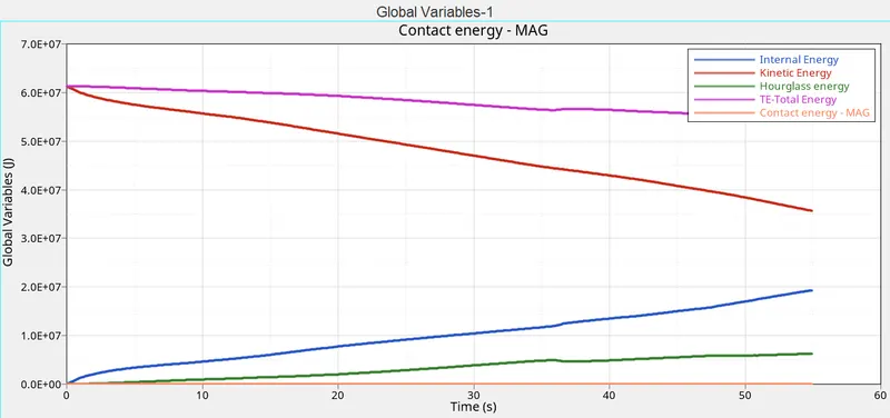
• It can be seen from the above image, that the kinetic energy decreases from the initial value, as the rate of beam movement towards the wall slows down.
• The internal energy, which is representative of the energy absorbed, increases and these energies approach convergence.
• Contact energy remains zero through out the simulation.

There is a bit of hourglass energy in the system, which is also responsible for the loss of energy (-10.3%), as the Q4 elements use Perturbation (viscous) method of hourglass control, which is more suitable for high deformation problems. This can be improved by using an element formulation with integrated hourglass control, or an external hourglass control card can be used.

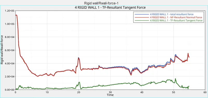
The rigid wall forces can be visualized as shown in the image below.

The maximum and minimum values of the displacement and the von-mises stress can be viewed in Hyperview and the buckling behaviour of the beam can also be visualized.

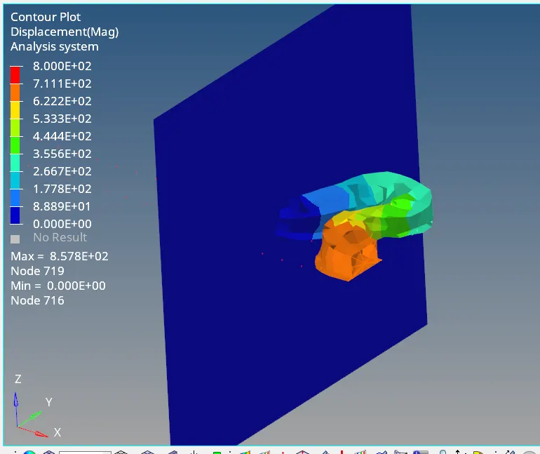
Plot of Displacement

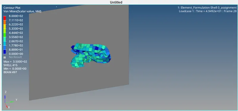
Plot of von mises stress

Simulation with recommended Element formulation

These results can be compared with the simulation results of the recommended element formulation.

The recommended parameters for the element formulation are as follows

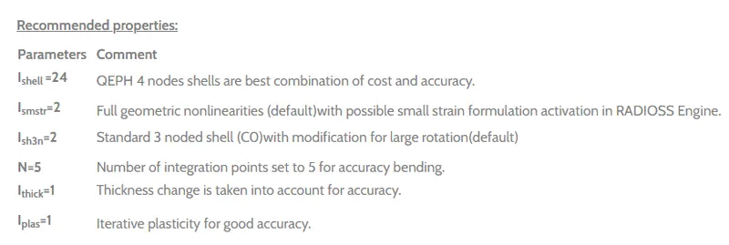
Step 1: Running the simulation

Modification of Run Time and Plot Frequency had done like previous step and The simulation with the recommended element formulation parameters has to be run using radioss. The recommended shell parameters are shown below.

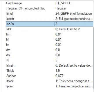
After the simulation is run, the results can be viewed in Hyperview and Hypergraph 2D.

Step 2: Results

The total energy and the mass error can be visualized from the 0001.out file at the end of the simulation.

The acceptable error limits are:

Energy error: -15% to +5%

Mass error: upto 2

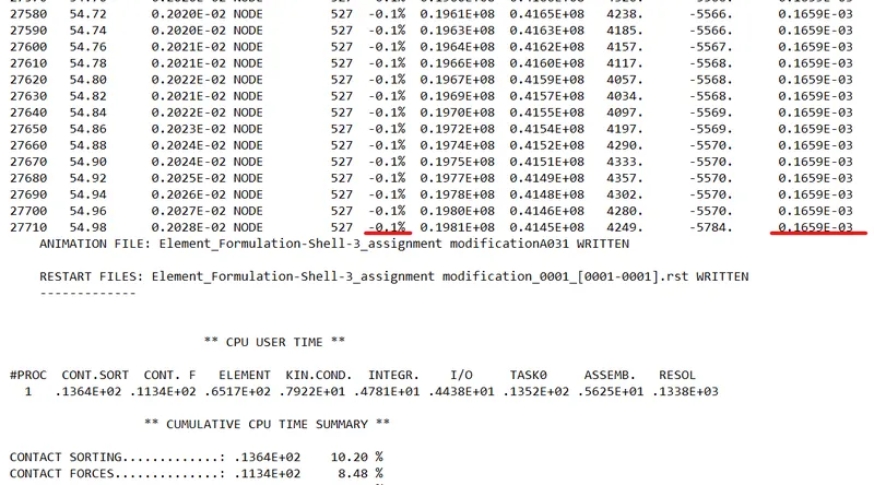
The energy error is -0.1% and the mass error is 0.1659 e-3, both of which are within acceptable limits.

The internal energy along with the hourglass, kinetic and total energies can be plotted in Hypergraph as shown below.

• It can be seen from the above image, that the kinetic energy decreases from the initial value, as the rate of beam movement towards the wall slows down.
• The internal energy, which is representative of the energy absorbed, increases and these energies approach convergence.

The hourglass energy in the system is close to zero, because the QEPH 24 elements have integrated hourglass control mechanism (stiffness method) to control the hourglass energy.

The internal energy along with the hourglass, kinetic and total energies can be plotted in Hypergraph as shown below.

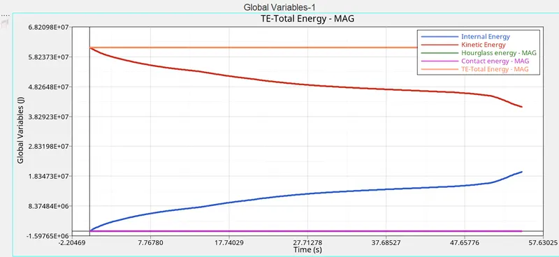
• It can be seen from the above image, that the kinetic energy decreases from the initial value, as the rate of beam movement towards the wall slows down.
• The internal energy, which is representative of the energy absorbed, increases and these energies approach convergence.
• Contact energy remains zero through out the simulation.
• Total Energy remains same throughout the simulation.

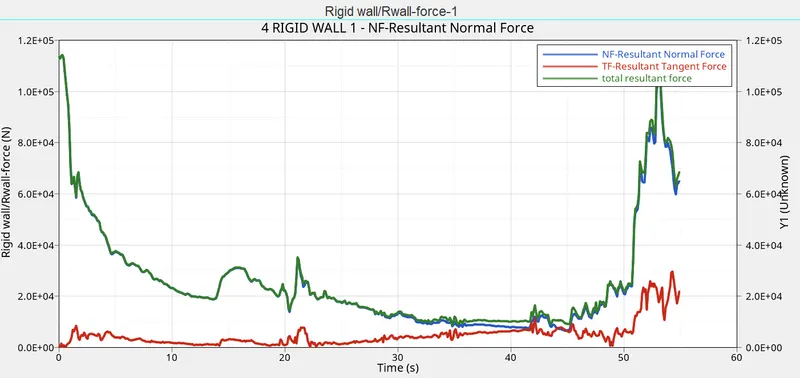
The rigid wall forces can be visualized as shown in the image below.

The maximum and minimum values of the displacement and the von-mises stress can be viewed in Hyperview and the buckling behaviour of the beam can also be visualized.

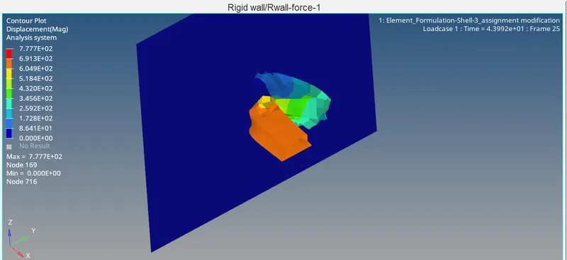
Plot of Displacement

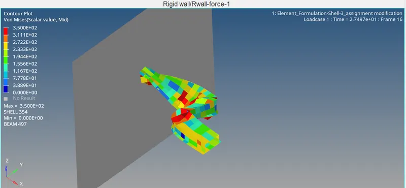
Plot of von mises stress

Comparison of Results

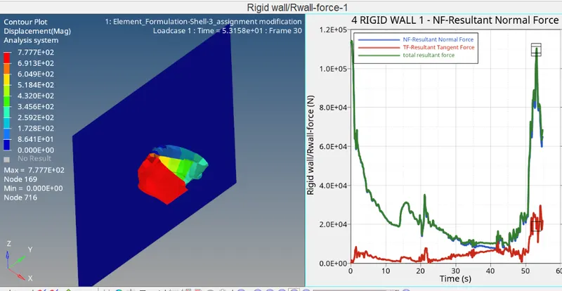
The following figures show the rigid wall forces of the base and the modified simulations.

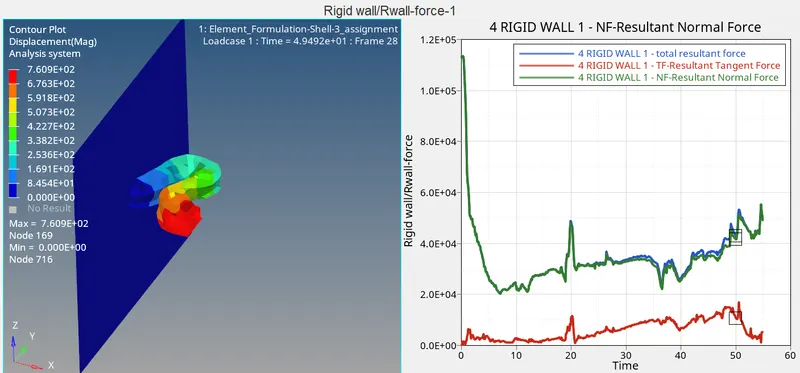
In the base simulation, the resultant rigid wall force remains fairly constant and increases slightly towards the end, as more area of the beam comes in contact with the rigid wall towards the end of the simulation.

In the modified simulation, the resultant force hits a peak towards the end at around 52 ms, since the rear part of the beam also comes into contact with the rigid wall due to the shape of the deformation, which results in a drastic increase in the normal force.

Energy and mass error

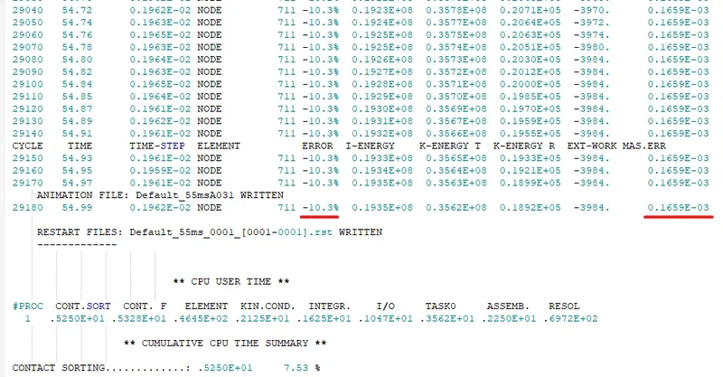
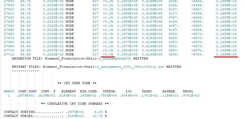
The error in the energy in the base simulation is -10.3% and -0.1% in the modified simulation. This is mainly due to the fact, that the Q4 elements used in the base simulation use Perturbation method of hourglass control, whereas the modified simulation makes use of QEPH 24 elements which has integrated hourglass energy control (stiffness method) as discussed below.

Hourglass energy

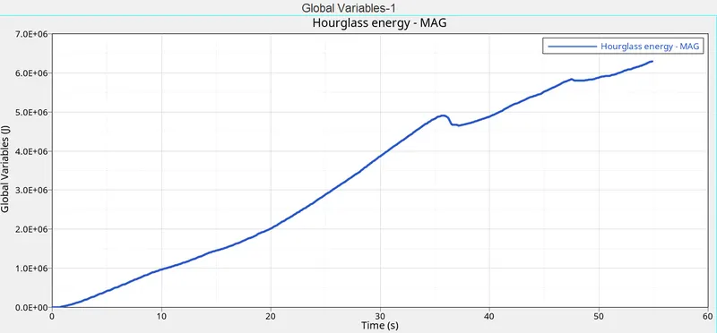
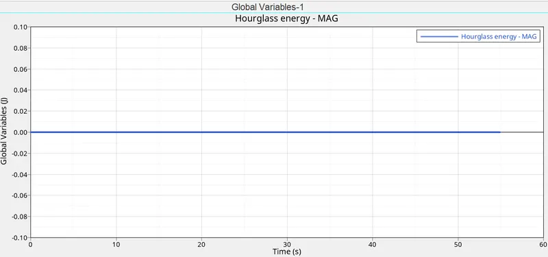
From the above image, it can be seen that the hourglass energy in the base simulation increases almost linearly with time, whereas it is zero in the modified simulation.

Total Energy

The image below shows the plots comparing the total energy in both simulations.

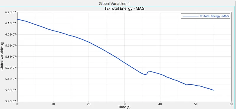
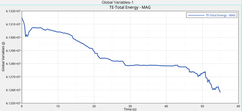
It can be observed, that the total energy at the end has a higher value in the modified simulation, since less of the energy is lost, due to the absence of hourglass energy. This further reinforces the improvement and the advantages that the QEPH 24 elements have over the Q4 elements, while maintaining similar levels of accuracy.

Conclusion

The comparative study on two different element formulations Q4 and QEPH 24 was extremely useful in providing insight on the differences between the two and helped gain an idea on the importance of choosing the right element formulation for the specific problem.