Assignment 5-RADIOSS Interfaces & Study of Effect of Notches Challenge

• Create the 2D mesh for bumper assembly and connect the crash box with bumper using connectors .
• mesh size should be 6mm.
• create different type of interfaces, assign recommended values to the interfaces and compare the base simulation setup results with different kinmatic condition simulation results.

1. Objective:

• To generate the mesh for the given bumper component with the mesh size of 6 mm.
• To change the parameters for the given crash tube model as various cases.
• To plot the graphs with RWALL forces, contact forces, internal energy (Post-processing) & compare the results.

Note:

• The widely used unit system in industries to develop a deck in the hypercrash is: KN, mm, ms, Kg.
• When a file is exported from the radioss( Hypercrash), It will create another new 0000.rad file. And it will store the previous 0000.rad file as a backup file(as 0000.rad.bak). And also it will create a M00 file(Which stores the data of tree & weld data).
• If that M00 file is deleted, In hypercrash we don't get the connection in our list of tree. But, they will be represented as a type 2 contact interfaces.
• In hyper crash, the engine cards are represented as control cards. And the data history file is seen in T01 file.

Interfaces (or) contact modeling:

The interfaces are defined as a model how the parts interact, when they come into contact with each other. While discussing the interfaces, there are four types of interfaces widely used. They are:

1. Interface penalty method
2. Type 7, Variable stiffness, Node to surface contact
3. Type 11, Variable stiffness, edge to edge contact
4. Type 24, Linear stiffness, node to surface & surface to surface contact

Other type is Type 19, which is the combination of both type 7 & type 11.

Penalty method:

This method treats the behavior between the slave nodes & master segments(surfaces) as springs that generate the resistive forces as a function of penetration, as shown in below figure.

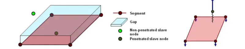
Time step is inversly proportional to the stiffness.

There are two types of time steps. They are:

• Nodal time step
• Kinematic time step

But the simulation is governed by the "Kinematic time step".

Type 7:

• This contact is used for node to surface contact.
• It can simulate all types of impact between a set of nodes and a master surface.
• It is non-oriented & slave nodes can belong to the master surface. Hence, the auto-impact is possible(can also be a self contact).
• In this method, the penalty method with variable stiffness can alos be used.
• Resistive forces are applied to keep the slave nodes out of the contact gap.
• Stiffness is non-linear.
• Contact gap can be constant or variable.

Contact gap: It's a gap between the slave nodes & master segment, which indicates when a slave enters in to that gap, which makes the resistive force come in to picture.

The resistive force vs penetration curve whivh is non-linear for the type 7 contact appears as shown in the below figure.

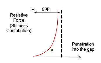
To have a stability, maintain the penetration lower level, which makes the stiffness less.

Important parameters in Type 7:

There are 7 parameters, which are important to be assigned at the time of creating the type 7 contact. They are:

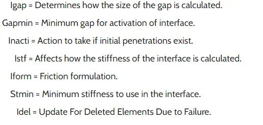
Igap: Which determines the size of the gap is calculated.

Gapmin: To indicate the minimum gap for the activation of interface.

Inacti: Action to take, if initial penetration exists.

Istf: Affects how the stiffness of the stiffness is calculated.

Iform:To indicate the formulation of friction.

Stmin: To indicate, how much minimum stiffness to be used in the interface

Idel: To indicate, what to do with the slave nodes & master segments if elements failed/deleted that they are attached to.

Igap:

Igap	Gap type	Description
0	Constant gap	The gap is defined by the Gapmin & is constant for all the contact. (Default)
1	Variable gap	Gap varies according to the characteristics of the impacted master surface & impacting slave node.
3	Variable gap	Variable gap with gap scale factor & mesh-size correction.

It depends on the Gapmin value (Recommended value for Gapmin is 0.5 mm).

Recommended value: 2 (or) 3

Reason: Majorly, used is 3. Because, gap scale factor & mesh size correction is taken in to account. Beacuse of adding gap scale factor, it puts a scale factor to the founded gap. In so many cases, there will be so many components with each other(i.e., By default the components will rest on each other). And if we don't want any reaction force to activate there. The Fscale gsp is going to relax the interface contacts by a bit. Which allows the slave node to reach up to the gap 0.8. Which reduces some calculations for solver.

Mesh-size correction: If the mesh size is big, then the nodes will be far away from each other. It is very likely, instead of nodes coming in to contact with the master segment, the edge of the slave node or element comes in to contact with the master. Because, the contact is not well defined. If the mise size correction factor, it can be overcomed.

Limitation of Type 7: It will consider only the nodes as a slave nodes.

Inacti:

Before discussing about Inacti, the initial penetration should be understood.

Initial penetration: Some nodes even pass behind or past to the master segment or element as shown in the below figure, which causes locking in simulations, leading to the computational failure.

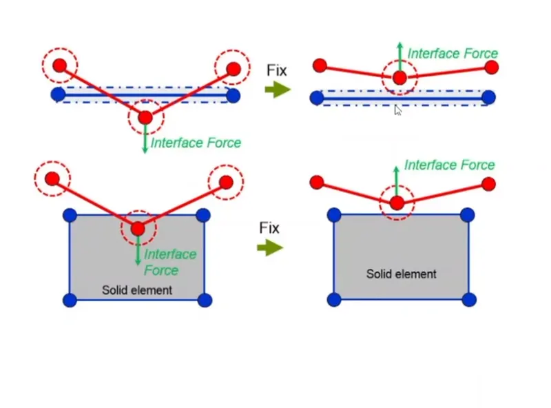
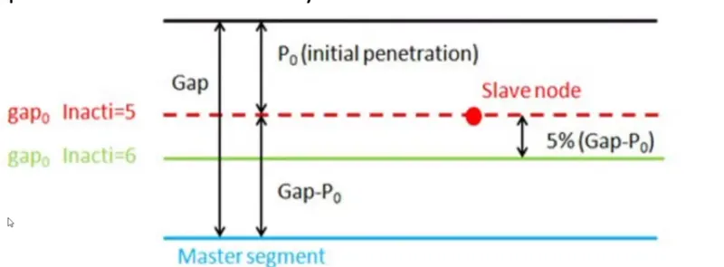
This can be overcomed by using a fix algorithm. After using it would be like, which puts a load on simulation, which leads to the pushing force going on this node, which results to the energy error in the simulation. There are so many values, and the recommended is 6, as shown in the below figure.

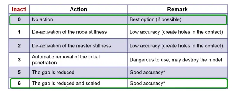
Reason: In case of going for value 5, it will scale down even further to as compared to case 5; the gap is reduced to P0 as shown in below figure. Becauseof that, In the case of vibrations at the slave side, the contact will get activated & deactivated. Which creates the problem. But where as in case of 6, it will scale scale down even further too, in such a way likeless than (Gap-p0). Which in dicates the less gap when compared to (Gap-p0) of inacti 5. This leads a slave node to vibrate. Because of sound wave propogation through it, which reduces the contact calculations & increases the stabiltity of simulation.

Istf:

The recommendes value is 4. The reason is: Because of mimimum stiffness, the resistive forces that are being applied on the slave node will be kept to minimum.

k = Max[stmin, min(stmax, Ko)]

where, Ko = min(Km, Ks); Km---> Stiffness of master segment, Ks---> Stiffness of slave nodes.

Example: If a soft component is coming in contact with a hard component, The soft component is going to absorb more resistive force & So that the stiffness of soft component should be considered. Beccause, the component is soft, it's stiffness is less. The final value for contact stiffness, can be bounded by lower(Stmin) & Upper limits (Stmax).

Iform:

Iform means "sliding force computation". The recommended value is Iform: 2.

Reason: Because the, sliding forces are computed using the stiffness parameters of the parameters. But whereas in Iform: 1, the sliding forces are computed using the viscous paramenters.

Idel:

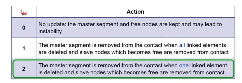
The parameter"Idel" indicates the update for deleted elements due to failure. The recommneded value is 2. The reason is shown in the below figure.

Finally the recommended values for the parameters are:-

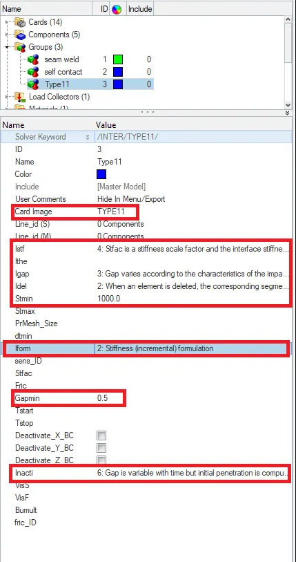
Igap = 2 (or) 3

Gapmin ≥">≥≥ 0.5 mm

Stmin = 1000 N/m (or) 1 KN/mm

Istf = 4

Inacti = 6

I del = 2

Iform = 2

Advantages & Disadvantages of Type 7 contact:-

Advantages:

• Physically correct representation
• High accuracy for describing the self contact & buckling.
• Best used with shells to shells (or) solids to shells.

Disadvantages:

• Requires more stringent modeling practices.
• Does not tolerate intersections(Slave node passing master segment).
• Time step may reduce due to increasing interface stiffness.
• With respect to the methodology, It will not see the contact due to edges crossing each other at angles.

Type 11 contact:

• It is also known edge to ege contact. In the case of edge crossing, type 11 interface can be added to capture the physics correctly.
• It is defined by identifying the master & slave lines in terms of edges.
• It works similar to type 7 contact interms of penalty formulation, gap definition, search method.
• Slaves will recieve stresses & forces. And the object which is to be analyzed is the "Slave".
• Coarser the mesh, stiffer the structure. Hence the master is typically meshed coarser. So that the slave doesn't penetrate in to the master. That's why the less deformable (or) highly stiffer structure is taken as master & less stiffer as slave.

Note: Type 19 contact is the combination of both type 7 & type 11 contacts.

Skew:

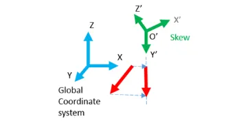
• Skew is one type of reference coordinate system which helps in defining local quantities with respect to the global coordinate system.

• Here the origin of the skew remains in a fixed position even if it is a fixed skew or moving skew.

• In a moving skew, the orientation of the node of interest is recomputed everytime, with that of the origin coordinates of the skew.

Application:- The example is the study of intrusions in the car through skews. 2 nodes are created and fixed skews are assigned to it. There the travel of the node is computed from the global coordinates and it is presented In the local coordinates. The overall travel of the node is obtained.

The skew is represented as shown in the below figure.

Frame:

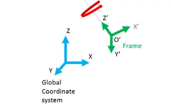
• A frame is a type of reference coordinate system where the quantities defined follow its own origin.

• Here, unlike the moving skew, the moving frame is attached with the node which is selected as origin.

• It helps in Calculating the motion of the body relative to the frame defined.

• Frames are used only in notable options like imposed velocity, imposed displacement, TH/node etc. The frame is shown in the below figure.

Tied contact/INTER/Type 2:-

Definition:- It is defined as an interface that kinematically connects a set of slave nodes to a master surface. It can be used to connect coarse & fine meshes, Model spot welds, rivets etc.

• Slave literally follows whatever the master is importing over the slave.
• Slave nodes can not have any motion by themselves. And if we put any constraints on the slave node except Type 2; it shows a pop-up like incompatible kinematic conditions.
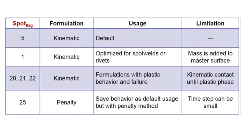
• It allows to use penalty method, which removes the potential incompatible kinematic conditions with the spot flag= 25. But in so many cases, Spot flag 25 is not recommended. Because, it will remove the errors automatiaclly, which may leads to arise new problems. The different formulation for spot flag is shown in the beow figure.

5. Procedure:

Model 1: Meshing the given model(Bumper):-

Initally, the user profile should be selected. As this model is to be only meshed. And hence no analysis is required, optistruct is selected is as an user profile...

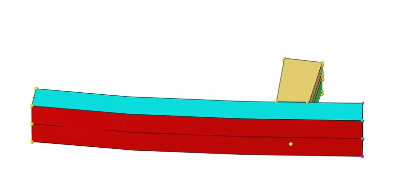
Then the model should be imported in the hyperworks software. After importing the geometry, the given geometry appears in the graphical display as shown

The next step is to view the component by topo. After switching it to topo, the geometry in the graphical display as shown

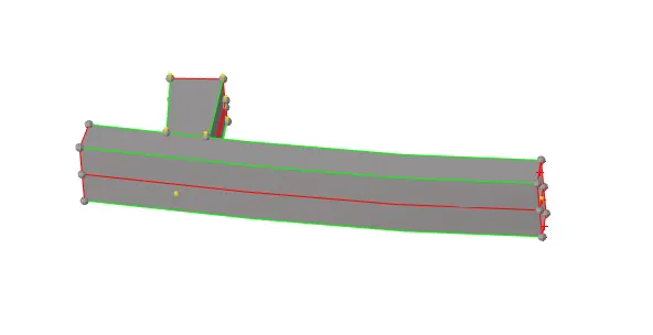
fig 5.3

Geometry clean up:-

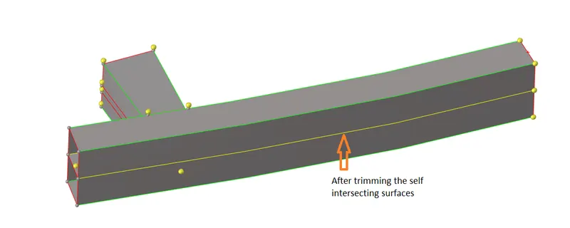
The next step is to clean up the geometry. In the given bumper model, there are some surfaces which are intersecting with each other. So, this can be overcomed by using the surface edit panel, trim with surfaces option

After trimming those self intersecting surfaces, the splitted surfaces will appear with yellow line(Indicating the juntion for three surfaces) as shownin

There are some surfaces which are to be connected as shown in fig by extending them.

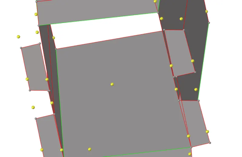
The extend option can be seen in surface edit panel, as shown in fig 5.7. In thet the line to extend over and surfaces to target should be selected.

After extending both the surfaces, the surfaces seems to be like self intersecting, as shown

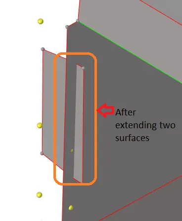
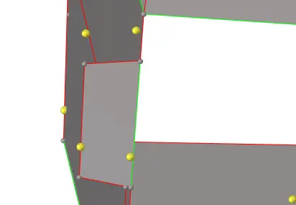
The next step is trim with the self intersecting surfaces. Then the extra surfaces are to be deleted. After deleting this extended surfaces, it appears as shown

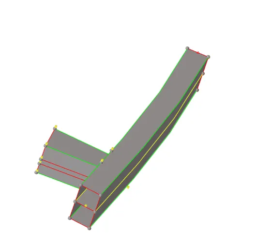
After geometry clean up, the given bumper model appears as shown

Meshing:-

Before meshing, the parameters as shown in fig 5.11 in the automesh panel should be selected. Anfd then by selecting the surfaces the by clicking on mesh, mesh will be generated.

After meshing, one surface. the mesh appears as shown

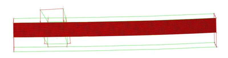
After meshing entire component, it appears as shown

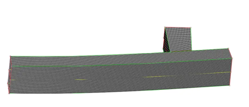
Then the given model(bumper) is connected with the help of rigid (RBE2) elements. Giving the connections depends on user. The process of selecting the rigid elements are: 1D panel---> Rigids---> selecting the nodes by switching to calculatie nodes. Selecting the nodes to form rbe2 elements is done as shown

After giving the connections between the sub-components, it appears as shown ...

v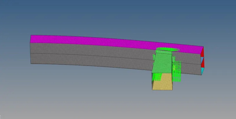

Model 2:(Performing various cases on the given tube model):-

Case 1:(Running the model as it is by defining the TH for interfaces):-

The next model is to analyzed. So, the user profile choosed is "Radioss" Then the starter rad(0000.rad) file should be imported, from the import solver deck option in the menu bar,

Case 1:(Running the model as it is by defining the TH for interfaces):-

1. import the cras box_0000.rad file in hypermesh using import solver deck option

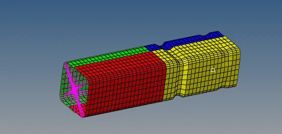
2. importent interface parameters

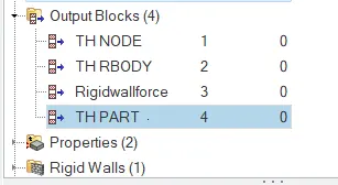
3. in order to create TH PART, we have to click on output blocks and create TH PART, in entity id instead of nodes change it to components and select all 4 components. hence TH PART is created

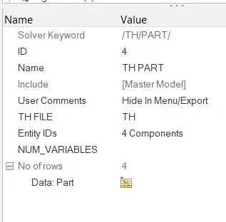
4. for this case dont change any paramter and run the simulation as it is

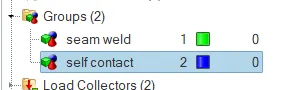
in hypermesh, go to - groups - self contact ( type7)

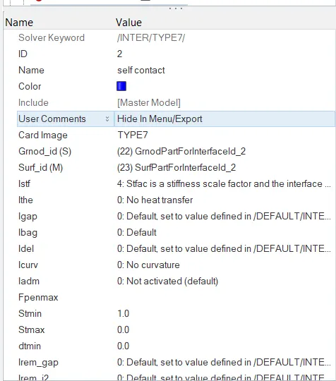
Then the simulation is to be runned. The process of running the simulation is: Analysis panel---> Radioss. As shown

Then the file should be saved in any location, Where all the animation files, time history files will be stored. And the "-nt 4" option is used to assign the task for the 4 cores in the cpu WHich will speed up the simulation.

Then by clicking on "Radioss", the simulation wil be runned. After some time, if the simulation is done properly and completed, it shows a pop-up as seen in fig Which indicates that, job is completed.

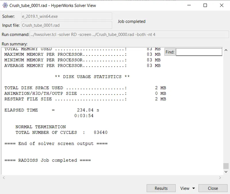
The created animation files in the specified location appears as shown in

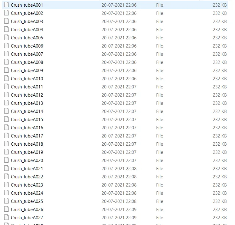
Then the 0001.out file is opened, to view the obatined results in the form of values. The obtained results for the last cycle is shown

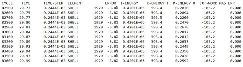
Then the next step is to simulate the model with respect to the obtained files. For doing that, the h3d file(combination of all animation files) is imported in the another window. After importing the h3d file, the given crash tube model with the rigid wall appears in the graphical display as shown

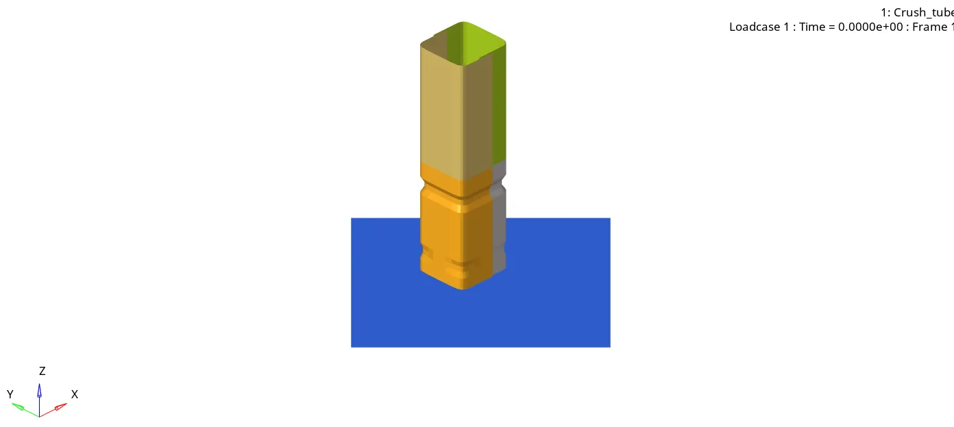
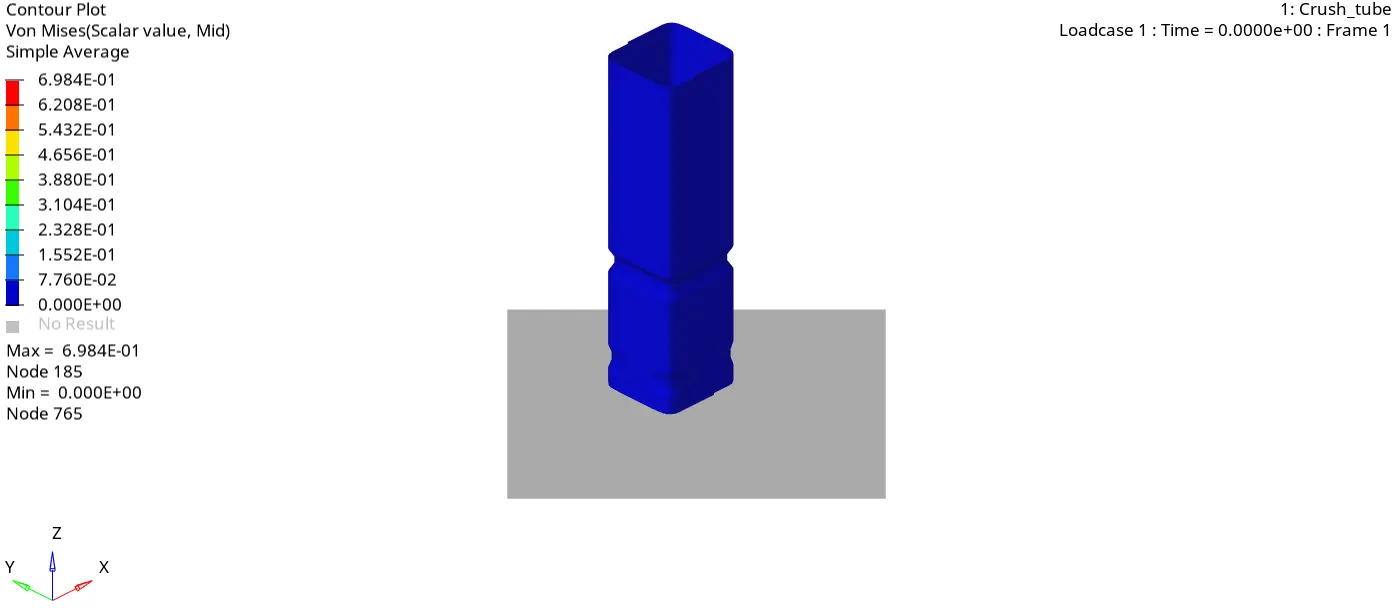
Then the contour panel is opened and the parameters such as result type, selecting the components & averaging method are selected. Then it is applied. The obtained simmulation in terms of von-mises, appears as shown in the below animation.

Post-processing:

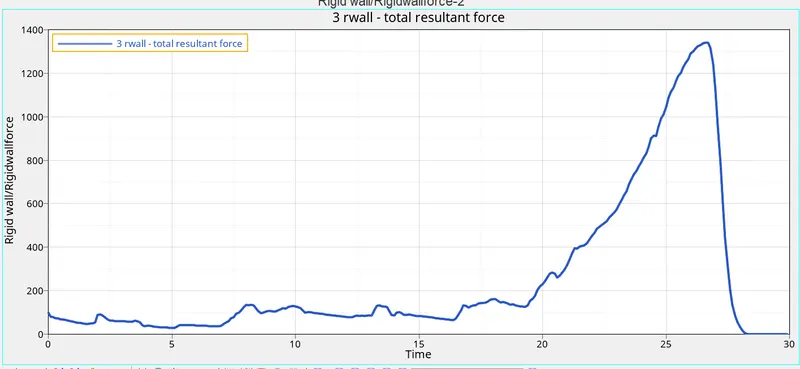
The next step is to do the post-processing(i.e., obtaining the graphs with the help of obtained results). For doing that, the T01 file should be imported in the other window. After importing the parameters should be selected to obtain the graphs. Initially, the rigid wall force graph is obtained. So, the parameters should be selected as shown

The obtained rigid wall force graph appears as shown It goes on increasing. Because, the forces with in the elements starts increasing at the beginning, when the velocity is given. And when the entire tube collides with the rigid wall, the rigid wall forces reaches to the peak value. Due to this the contact energy increases, which results the increase in rigid wall forces.

The obtained contact force graph appears as shown Initially, there will be no contact forces at the beginning. So, the curve starts from origin. And there will be some fluctuations in the curve at the middle. Due to fluctuation of contacts with in the elements. And then it reaches to the peak value as shown in , when the entire model undergoes collision, there will be more contact with in the elements & even with rigid wall.

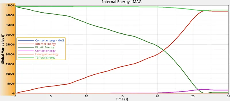
The obtained internal energy graph appears as soon The internal energy increases to the peak value at the end of the collision. And becomes constant. The Kinetic energy which is having higher value at the start of the simulation decreases as the simulation progresses with time and gets converted to internal energy, thus internal energy increases with time. The Total energy in the system is almost constant where the slight decrease is due to the energy error which is caused due to the resistive forces between master segment and slave nodes.

Case 2:(Changing the inacti value to 6):-

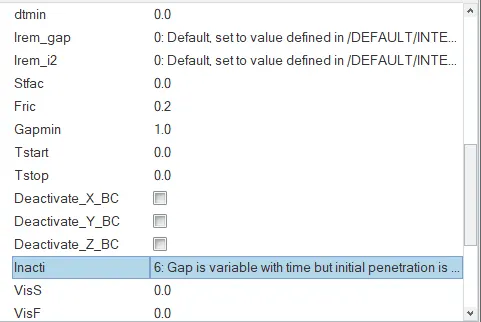
In this case, In the interfaces card the inacti value is changed to 6[INTER>TYPE 7 in SOLVER BROWSER], as shown in Then, the simulation is runned. With this, the gap will be scaled further in between the slave & master.

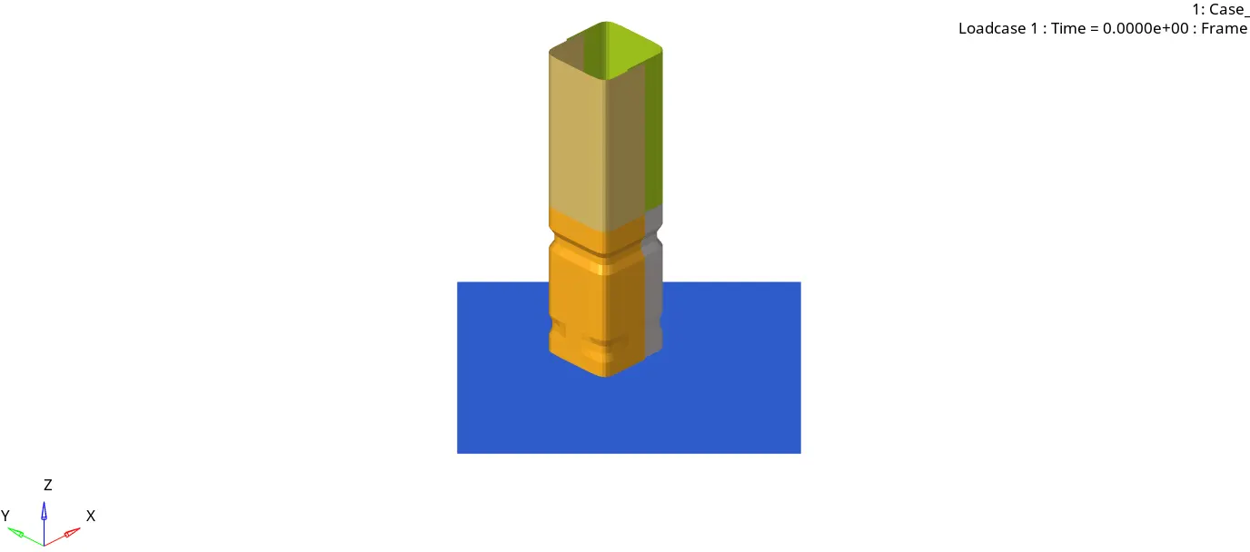
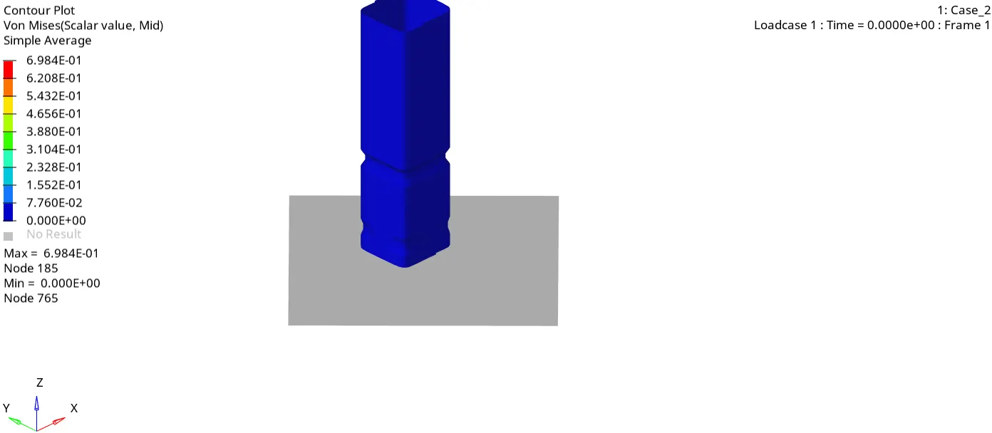
Then the obtained simulation from h3d file in terms of von-mises stress appears as shown in the below animation.

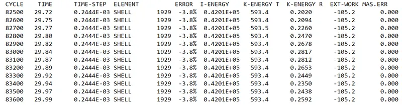
After running the simulation, the obtained 0001.out file is opened. To view the obatined results in the form of values. The obtained results for the last cycle is shown in

Post-processing:

Then the To1 file is opened in another window. Inorder to view the results in terms of graphs. The obtained rigid wall force graph appears as shown It goes on increasing. Because, the forces with in the elements starts increasing at the beginning, when the velocity is given. And when the entire tube collides with the rigid wall, the rigid wall forces reaches to the peak value. Due to this the contact energy increases, which results the increase in rigid wall forces. It will be some what similar to case 1.

Then the graph to be obtained is, contact forces. The obtained contact force graph appears as shown in Initially, there will be no contact forces at the beginning. So, the curve starts from origin. And there will be some fluctuations in the curve at the middle. Due to fluctuation of contacts with in the elements. And then it reaches to the peak value as shown in when the entire model undergoes collision, there will be more contact with in the elements & even with rigid wall. It will aslo be some what similar as in case 1. Becuase, there are no initial penetrations.

Then the internal graph is obtained. The obtained internal energy graph appears as shown in The internal energy increases to the peak value at the end of the collision. And becomes constant. As there is no change in the above graphs, there is change in internal energy graph also.

Case 3:(Creating the type 11 contact):-

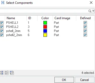
In this case, the new contact named "Type 11". In this contact, some parameters are to be entered, as shown in In order to get, the better results.

While defining the slaves & master, ensure that all elements should be as a slave & as well as master, as shown in fig 5.40.

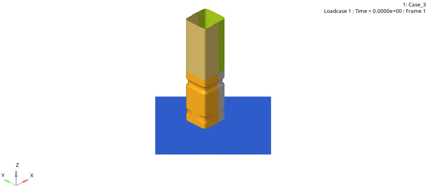
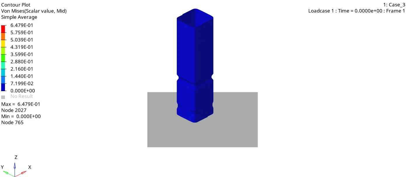
The next step is to run the simulation. After running the simulation, the obtained simulation from h3d file in terms of von-mises stress appears as shown in the below animation.

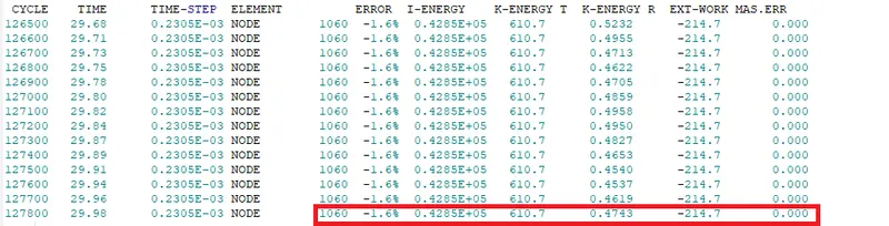
After running the simulation, the obtained 0001.out file is opened. To view the obatined results in the form of values. The obtained results for the last cycle is shown

Post-processing:

Then the post-processing is done. The obtained rigid wall force appears as shown in Frome that graph, The thing noticed is the rigid wall force value is increased (With in the range 1400-1600), when compared to the previous cases. The reason is, Type 11 contact is also defined along with the pre-defined type 7 contact. So, the contact forces with respect to the edge to edge contacts are also seen.

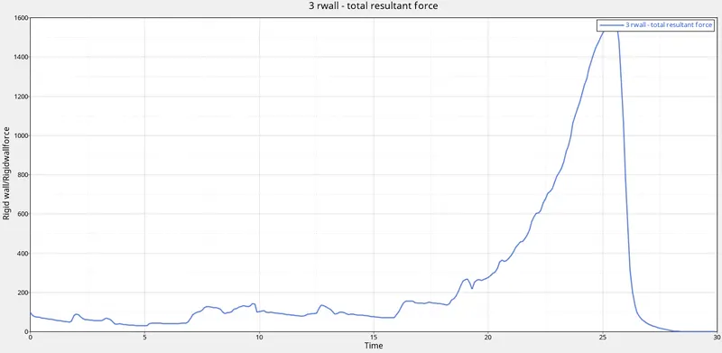
The next graph obtained is, contact forces with respect to type 7 contact. The obtained contact forces graph for type 7 contact is shown . The contact forces will be constant and reaches to the peak value, when all of a sudden the nodes comes in contact with the master elements with in the tube model. And the graph falls back, when the model attains reaction against the rigid wall.

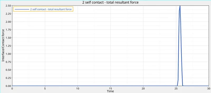
Then a graph is obtained for the type 11 contact. The obtained graph for type 11 contact is shown in . As this graph depicts about the edge to edge contact. There will be the fluctuations, as the edges of the elements comes in to contact gradually. ANd reahes to a peak value, after the entire collision. And decreases thereby due to the little expansion of the model after hitting the rigid wall.

Then a graph is obtained for the internal energy, which appears as shown in fig . There will be no change in the kinetic energy.

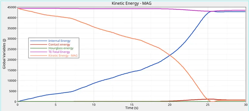
The internal energy increases linearly as the deformation progresses and it goes in a constant value once the deformation is completed. Similar to the previous case the contact forces also increases linearly and reaches the maximum value at the highest deformation stage and it falls down once the maximum deformation has crossed and maintains a constant value.

The rigid wall forces were similar to the other case however the tangent resultant force seems siginificantly higher than the other cases with the usage of Type 11 interface.

CASE 4: IMPORT THE STARTER FILE AND REMOVE ALL THE NOTCHES AND REMOVE BOUNDARY CONDITIONS

Import the model

After importing remove all the notches by using project and allign command and also remove boundry conidition

For that

Go to Solver browser >> Delete Boundry condition (BC) OR enable DOF's

Now save the file into the folder and run

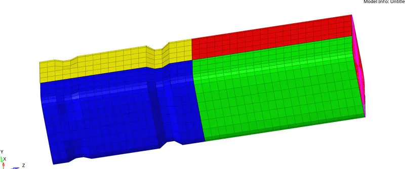
NOTCHES IN MODEL

Remove this two notches

PROJECT TAB

ALLIGN NODE

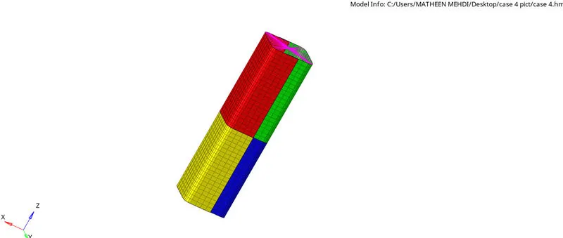
NOTCHES REMOVED

After removing boundry condition save the model and run

Once the simulation done, Open engine out file write down all the value

Here are the output values, which are acceptable numbers: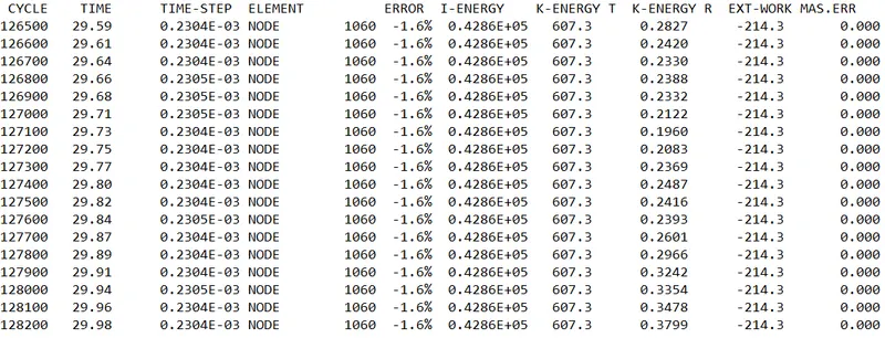
]

Now open the animation

For that

Go to Hyperveiw >> Select animation file >> Apply

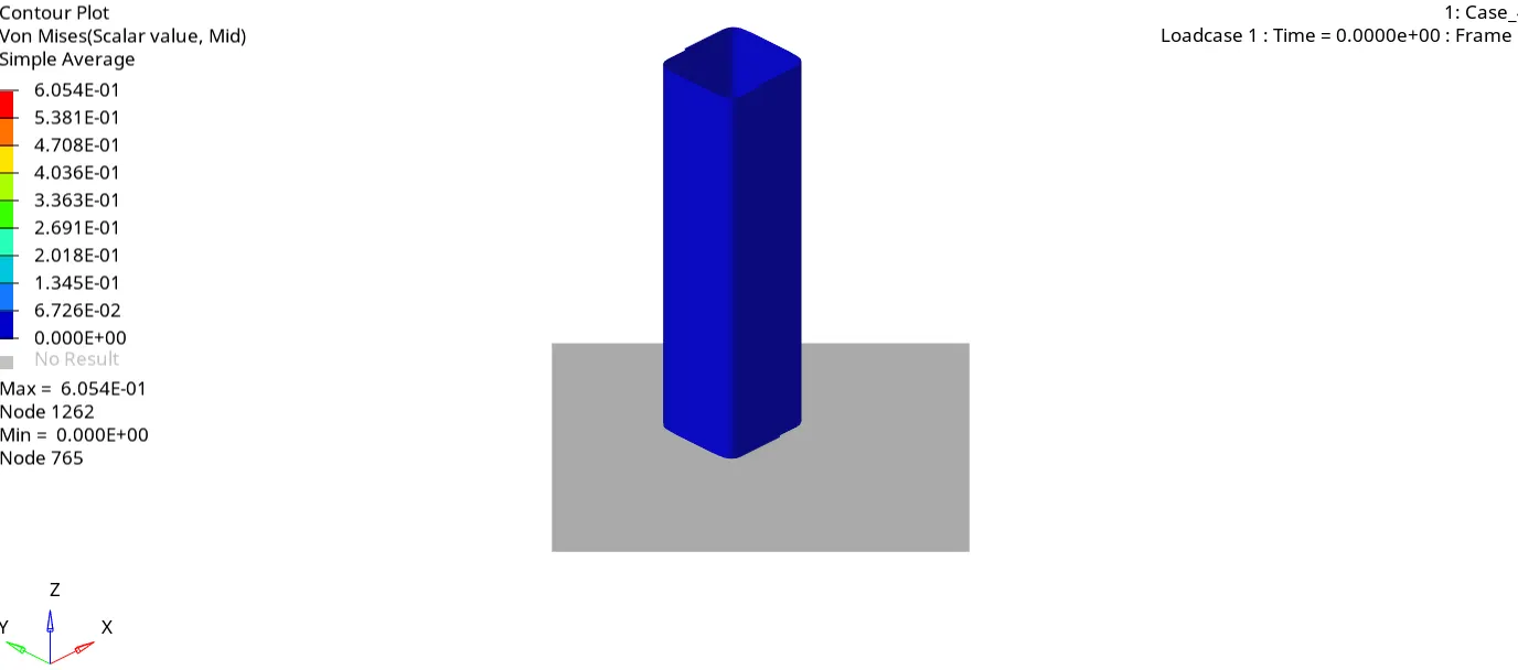
To see von-mises

Go to contour in hyperveiw >> Select von-mises >> Select: Simple >> Apply

Energy Plot

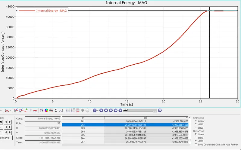
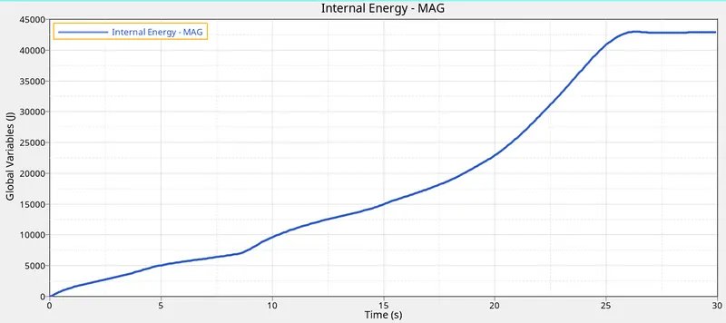
The internal, kinetic, hourglass and the total energies can be plotted using the TO1 file in Hypergraph 2D, as shown below.

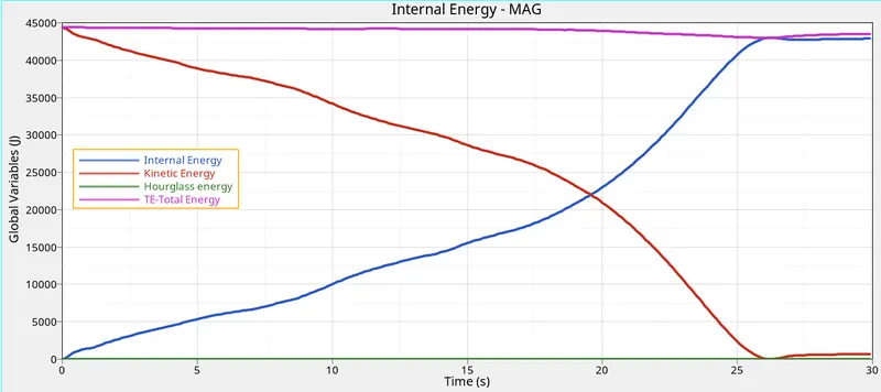
The internal energy, which is representative of the energy absorbed, increases with time, as the tube makes contact with the rigid wall. We can observe a small peak and a drop off at around 27 seconds, which is the time when the tube is completely crushed and no more energy can be absorbed by the system.

The hourglass energy is zero, since the QEPH 24 element formulation has integrated hourglass control.

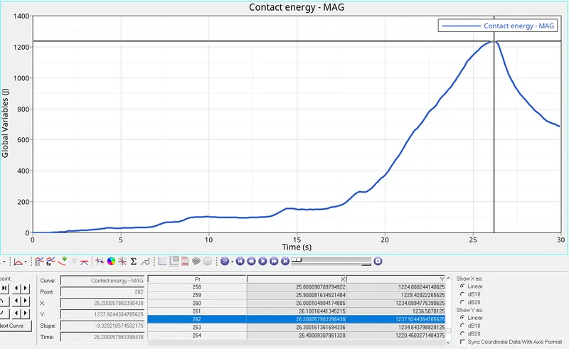
Internal and Contact energies

The plots below show the maximum values of the internal and the contact energies.

The max internal energy is 42980.28

The max contact energy is 1237.92

RIGID WALL FORCE

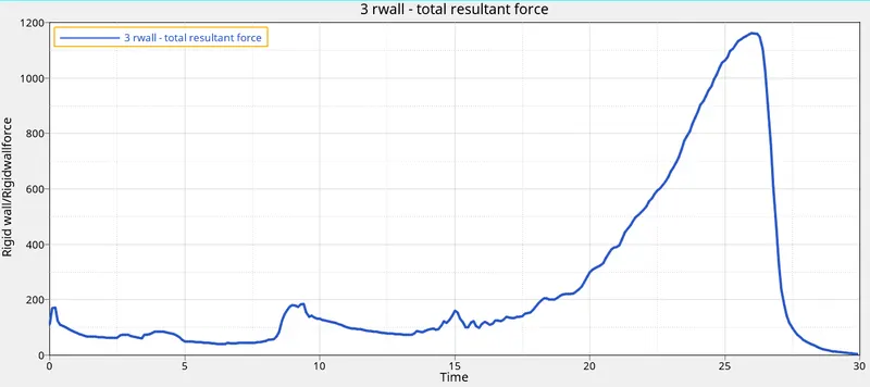
The force on the rigid wall due to the impact, over the course of the simulation is shown in the figure below.

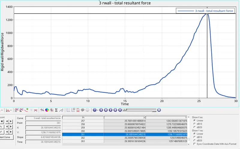
The max force is 1296.71 N, which coincides with the point at which the the internal energy peak is achieved. This represents the point in the simulation, at which the crush tube is completely deformed, and the rigid wall has to react the forces due to the impact motion of the rigid body.

The value of the force drops rapidly thereafter, since the entire crush tube bounces away after the impact and loses contact with the rigid wall.

CASE 5: Create a new notch in the middle, select the whole section and run

For this case, we shall be using the starter file of case 4. So there are no notches or boundary conditions. But the case requires us to create a notch through the middle section of the crush tube. For this, we shall be making use of the translate tool in Hyperworks. After importing the starter file in Hyperworks, we can go to tools > translate.

We can either select elements or nodes to translate. After assigning the direction of translation (using an axis or a vector), we then need to assign a magnitude. Depending on the global axis, we then have to either click 'translate+' or 'translate-'. This creates the depression.

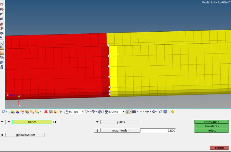
After creating Middle notch

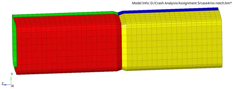
Now, we need to run the analysis through the radioss engine and generate the simulation. This is what it looks like:

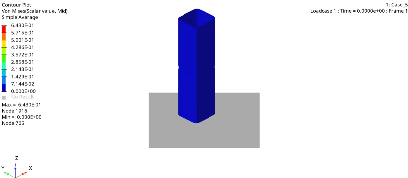
Just as in the first 3 cases, the notch is the region where the tube undergoes deformation first. Then the region closer to the rigid wall is deformed next, which would be the lower half of the tube. Around the 10-12ms mark, when the lower half is mostly deformed, the upper half undergoes proper, visible deformation very rapidly until the entire tube is crushed completely. In addition to that, based on the nature of the notch, there may be anomalies. Since it was created manually.

Taking a look at the readings in the output file, we can see that the values are acceptable: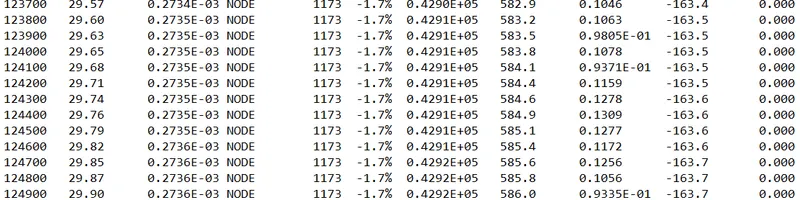

Moving on to the energy and rigid wall plots:

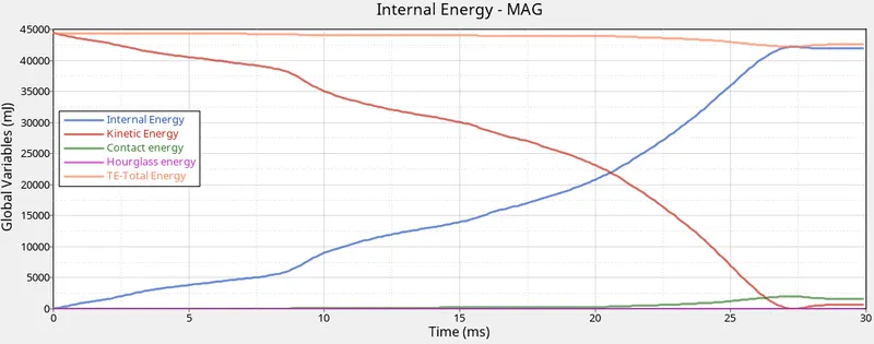
Contact energy:

• Contact Energy is the energy acting opposite to the system to prevent the penetration acting on the system. When the force is applied to the body, the crush tube starts to deform but the penetration happening is low in the initial stage. The contact energy will below.
• Once the deformation is maximum, the elements will be forced to penetrate but the opposite force which is contact energy will also increase which helps in the prevention of penetration. Once the deformation ends, the contact energy will become zero and will stay constant thereafter.
• In this case, the contact energy incurred is more when compared to case 1 and case 2. This is due to only one notch at the center which increases the rate of deformation, which intern increases the rate of penetration.

• The obtained graph for internal energy. There will be a change in the internal energy. Because, As there is a notch only at the middle. The elements will be impacted without any deviation, as of in the previous cases in which the notch is present at the beginning. There will be a drop in the internal energy at the middle as shown in fig. Due to the model moves back after hitting the rigid wall. And there will be a rise again. Because the model again hits with the elements after notch.

CASE 6: Create a new notch with nodes only from opposing 2 faces and run

• In this case, the new notch is created in the middle again. But only at the two opposite faces.

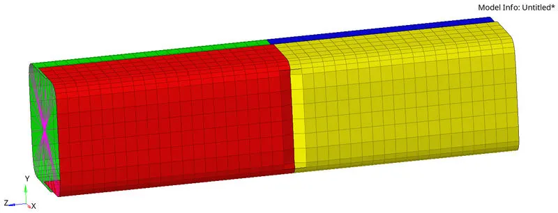
We can then carry out the analysis using radioss as outlined in the main procedure. The simulation is as follows:

• Then the obtained 0001.out file is opened. To view the obtained results in the form of values. The obtained results for the last cycle

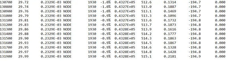
They have acceptable energy and mass error values.

• Then the simulation is run. After running the simulation, the obtained h3d file is imported into hyperview to view the simulation. The obtained simulation appears as shown in the below animation.

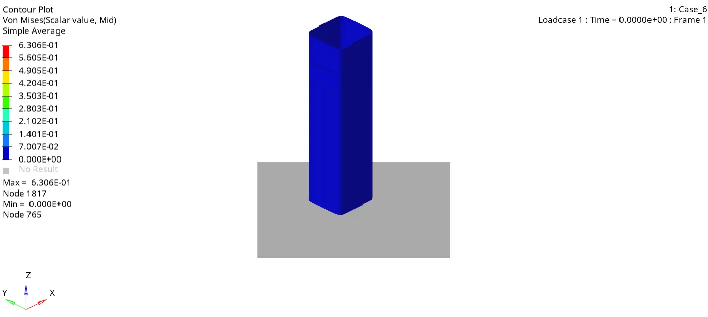
• Deformation takes at the middle notch of the model due to applied velocity due to stress concentration near the notch
• After complete deformation of the notch. The next deformation occurs at the bottom which is near to the Rigid wall is because the thickness is less at the bottom which is 2.1mm

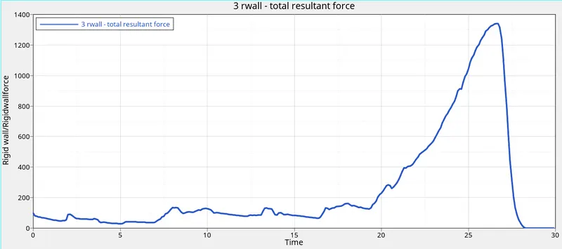
• Rigid wall force

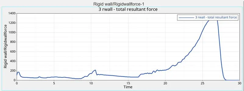
The max force is 1361.06 N, which coincides with the point at which the the internal energy peak is achieved. This represents the point in the simulation, at which the crush tube is completely deformed, and the rigid wall has to react the forces due to the impact motion of the rigid body.

The value of the force drops rapidly thereafter, since the entire crush tube bounces away after the impact and loses contact with the rigid wall.

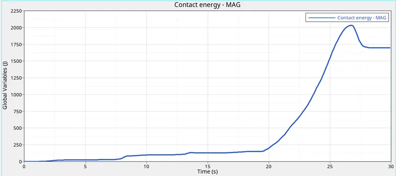
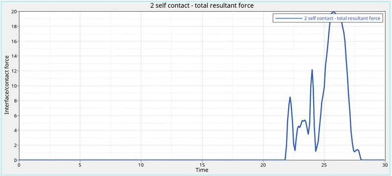
• contact force

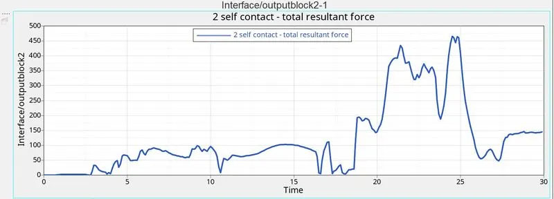
It can be observed, that the self contact energy has a peak at around 20 seconds, when most of the tube is completely deformed. We can see a secondary peak at around 24 seconds, which is due to the tube being fully compressed at this point, which leads to maximum contact of between adjacent elements.

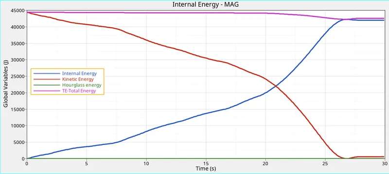
• Energy plot

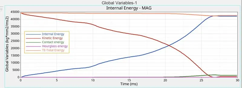
The internal energy, which is representative of the energy absorbed, increases with time, as the tube makes contact with the rigid wall. We can observe a small peak and a drop off at around 27 milli seconds, which is the time when the tube is completely crushed and no more energy can be absorbed by the system.

The hourglass energy is zero, since the QEPH 24 element formulation has integrated hourglass control.

OBSERVATIONS AND RESULT

Notches are the regions where deformations happen first , due to them being regions of stress concentration. But it does help to control and predict the location of deformations. This in turn plays a role in how the absorbed energy spreads throughout the tube. A notched tube results in higher contact forces but a smoother transmission of load.

In this assignment, different types of contacts were used to analyze the simulations of the crash tube. Under a constant load, the behaviour was observed by varying the geometry through the removal and creation of notches.