Air standard Cycle(Otto cycle) using MATLAB

Objective: -

Develop a program that can solve an otto cycle and make a plot for it.

Principle: -

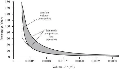
An Otto cycle is an idealized thermodynamic cycle that describes the functioning of a typical spark-ignition engine. It is the thermodynamic cycle most commonly found in automobile engines. The Otto Cycle is an air-standard cycle that approximates the processes in petrol or diesel engines. It is based on constant volume heat addition (combustion) and heat rejection processes, and Isentropic compression and expansion

There are three air-standard cycles:

• constant volume ‘combustion’ (Otto)
• constant pressure ‘combustion’ (Diesel)
• dual ‘combustion’ – this is a combination of constant volume and constant pressure combustion and results in a slightly more realistic cycle.

Solution Procedure: -

The basic Otto cycle has four processes:

•Isentropic compression

•Constant volume heat addition

•Isentropic expansion

•Constant volume heat rejection

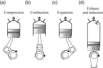
Processes: -

• Process 0 - 1 Intake Stroke
• Process 1 - 2 Compression Stroke
• Process 2 - 3 Ignition Phase
• Process 3 - 4 Expansion Stroke
• Process 4 - 1 Idealized Heat Rejection
• Process 1 - 0 Exhaust Stroke

Governing Equations: -

• Change of Volume Inside the combustion chamber of an engine -

`(V)/(Vc)=1+0.5(CR-1)[R+1-cosθ-(R^2-sin^2 θ)^0.5]`

• Isentropic Process

`PV^r=constant`

• Isenchoric Process

`P/T = constant`

• Compression Ratio

`CR = (Vs + Vc )/(Vc)`

• Thermal Efficiency

`η=1-1/(RC)^(γ-1)`

CODE for the Function: -

%Function for calculation Volume compression and expression

function[V] = engine_kine(bore,stroke,con_rod,cr, st_crank,end_crank)
cr =12
%Crank pin radius = stroke/2 in meter

a=stroke/2

%Ration of connected rod to the crankpin radius 

R = con_rod/a

%Swept volume and Clearance Volume in (m^3)

v_swept =pi/4*bore^2*stroke;
v_c= v_swept/(cr-1)


theta = linspace(st_crank,end_crank,100);

term1=0.5*(cr-1);
term2 =R+1-cosd(theta)
term3= (R^2 - sind(theta).^2).^0.5;

V= (1+term1*(term2 -term3)).*v_c;

end

Explanation of the above code: -

• % - comments to make the code user friendly
• function[V] = engine_kine(bore,stroke,con_rod,cr, st_crank,end_crank)

function is used to make the code easy to implement ,it is a group of statements that together perform a task

• cr =12 - initializing compression ratio as 12
• a=stroke/2

a is equal to crank pin radius which is equal to stroke/2

• R = con_rod/a - Ration of connected rod to the crankpin radius
• v_swept =pi/4*bore^2*stroke - Swept volume in (m^3)
• v_c= v_swept/(cr-1) - Clearance Volume in (m^3)
• theta = linspace(st_crank,end_crank,100) - used to create a volume array than a pressure array
• term1=0.5*(cr-1);
• term2 =R+1-cosd(theta)
• term3= (R^2 - sind(theta).^2).^0.5;
• V= (1+term1*(term2 -term3)).*v_c; - calculation using all above term
• end - to close the function

Code of the Otto cycle Program: -

clear all
close all
clc
%inputs
gamma =1.4
t3 =2300
% State variable
p1 = 101325
t1 = 500

% Engine geometric parameters
bore= 0.1;
stroke = 0.1;
con_rod = 0.15;
cr= 12;

%calculating the swept volume and clearence volume
v_swept =(pi/4)*bore^2*stroke;
v_clearance= v_swept/(cr-1);

v1 = v_swept + v_clearance
v2 = v_clearance

% state variables at state point 2
%p2v2^gamma = p1v1^gamma 
%p2 = p1*(v1/v2)^gamma = p1*cr^gamma
p2= p1*cr^gamma;

%p1v1/t1 = p2v2/t2 | t2 =p2*v2*t1/(p1*v1)
t2 =p2*v2*t1/(p1*v1);

constant_c=p1*v1^gamma;

v_compression = engine_kine(bore,stroke,con_rod,cr,180,0);

%p_compression*v_compression^gamma = constant_c
p_compression = constant_c./v_compression.^gamma ;
% state variables at state point 3
v3 = v2
%p3v3/t3 = p2v2/t2 | p3 =p2*t3/t2
p3 = p2*t3/t2
constant_c= p3*v3^gamma;
v_expansion = engine_kine(bore,stroke,con_rod,cr,0,180);
p_expansion = constant_c./v_expansion.^gamma;

% state variables at state point 4
v4=v1;

%p3v3^gamma = p4v4^gamma | p4 = p3(v3/v4)^gamma
p4 = p3*(v3/v4)^gamma;

%Thermal Efficiency
thermal_effi = 1-((cr)^(1-gamma))

figure(1)
hold on
plot(v1,p1,'*','color','r')
plot(v_compression,p_compression)
plot(v2,p2,'*','color','r')
plot(v3,p3,'*','color','r')
plot(v_expansion,p_expansion)
plot(v4,p4,'*','color','r')
plot([v1 v_compression v2 v3 v_expansion v4 v1],[p1 p_compression p2 p3 p_expansion p4 p1],'color','b')

grid on
title('Air Standard Cycle : Otto Cycle')
xlabel('Volume')
ylabel('Pressure')

Explanation of the above code: -

• clear all - to clear all the workspace variables
• close all - to close all the output window
• clc - to clear the command window
• % - comments to make the program user friendly
• gamma =1.4 - to initializing gamma with 1.4
• t3 =2300 initializing to as 2300 kelvin
• p1 = 101325 initializing p1 as 101325 pascal
• t1 = 500 - initializing t1 as 500 kelvin

Engine geometric parameters

• bore= 0.1 - initializing with 0.1 meter
• stroke = 0.1 - initializing with 0.1 meter
• con_rod = 0.15 - initializing connecting rod length as 0.15 meter
• cr= 12 -initializing compression ration as 12

calculating the swept volume and clearence volume

• v_swept =(pi/4)*bore^2*stroke - calculating the swepth volume
• v_clearance= v_swept/(cr-1) - calculating the clearance volume
• v1 = v_swept + v_clearance - calculating v1 volume
• v2 = v_clearance - calculating v2 volume

state variables at state point 2

• p2= p1*cr^gamma; - calculating p2 pressure
• t2 =p2*v2*t1/(p1*v1); - calculating temperature t2
• constant_c=p1*v1^gamma; - calculating constant c
• v_compression = engine_kine(bore,stroke,con_rod,cr,180,0); - calling of the function to calculate compression volume
• p_compression = constant_c./v_compression.^gamma ; - calling of the function to calculate compression pressure

state variables at state point 3

• v3 = v2 - initializing volume v3 volume v2
• p3 = p2*t3/t2 - calculating p3 pressure
• constant_c= p3*v3^gamma; - calculating c constant for expansion processes
• v_expansion = engine_kine(bore,stroke,con_rod,cr,0,180); - calculating expansion volume
• p_expansion = constant_c./v_expansion.^gamma; - calculating expansion pressure

state variables at state point 4

• v4=v1; - initializing volume v4 volume v1
• p4 = p3*(v3/v4)^gamma; - calculating p4 pressure

%Thermal Efficiency

• thermal_effi = 1-((cr)^(1-gamma)) - calculating theraml efficiency of the otto cycle
• figure(1) - to open a new plot window
• hold on - to hold the plot
• plot(v1,p1,'*','color','r') - plotting of the point v1 volume and p1 pressure
• plot(v_compression,p_compression) -plotting of the point of compression volume and compression pressure
• plot(v2,p2,'*','color','r') - plotting of the point v2 volume and p2 pressure
• plot(v3,p3,'*','color','r') - plotting of the point v2 volume and p3 pressure
• plot(v_expansion,p_expansion) - plotting of the point of expansion volume and expansion pressure
• plot(v4,p4,'*','color','r') - plotting of the point v4 volume and p4 pressure
• plot([v1 v_compression v2 v3 v_expansion v4 v1],[p1 p_compression p2 p3 p_expansion p4 p1],'color','b') - plotting of the graph
• grid on - to show the grid
• title('Air Standard Cycle : Otto Cycle') - to give the title to the plot
• xlabel('Volume') - to initialize x ais
• ylabel('Pressure') - to initialize y axis

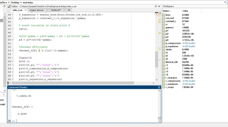
Output : -

Thermal efficiency in the command window

The workspace variables

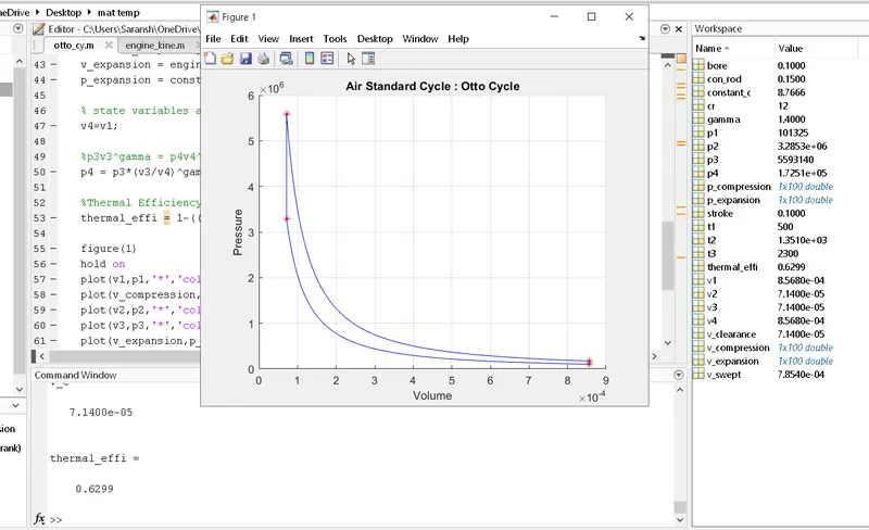
The output plot of the otto cycle: -

Conclusion and Discussion: -

• Thermal Efficiency was calculated to be 0.6299 or 62.99%.
• The graph was plotted between Pressure and volume for an otto cycle.
• The Air standard efficiency depends on the compression ratio.