WOT Condition
AIM:- To understand the Wide Open Throttle(WOT).
OBJECTIVE:- To understand the Wide Open Throttle(WOT) Conditions on a vehicle and answer the following questions.
# Ques-1 Calculate the ratio of hill-climbing power required by a fully loaded tata ultra truck to the half-loaded one.
Given Data- For this question I am taking the details of the TATA T.16 ULTRA truck
Kerb weight = 6255 kg
Payload Capacity = 9765 kg
GVW(Gross Vehicle weight) = Kerb weight + Payload Capacity
m = GVW = 6255 + 9765 = 16020 kg
g = 9.81
Hill Climbing Angle = 10° (assumed)
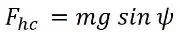
HIll Climbing Force - Hill Climbing Force is the ability of a vehicle to climb on a typical hill or slope at a given constant speed.
Usually upgradient(upwards) is considered for vehicle performance analysis
Hill Climbing Force can also be represented as Gradability of vehicle
| Fully Load Condition | Half Loaded Condition |
| m1 = 16020 kg | m2 = 11133 kg |
|
Hill Climbing Force = 16020 * 9.81 * sin(0.174533) = 27289.899 |
Hill Climbing Force = 11133 * 9.81 * sin(0.174533) = 18964.946 |
| Hill Climbing power (At constant speed) P1 = F1*v |
Hill Climbing power (At constant speed) P2 = F2*v |
|
= 27289.899 * 80 = 2183191.92 |
= 18964.946 * 80 = 1517197.12 |
The ratio of hill-climbing power required by a fully loaded tata ultra truck to the half-loaded one is-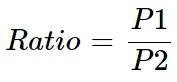
Ratio = 2183191.92 / 1517197.12 = 1.43896
# Ques- 2 Calculate the minimum length of the flyover.
A flyover is planned to be constructed on a national highway. Keeping in mind the Gradeability for trucks, how much can be the minimum length of the flyover,
considering the minimum height at the summit should be 5.5 meters.
Given:-
Rise = 5.5 m
Gradeability= Taking the Gradeability of TATA T.16 ULTRA truck (25.2%) 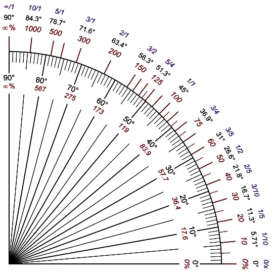
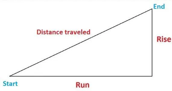
For 25.2% Gradeability the maximum slope angle is 15°
Length of Flyover = `(Rise) / Sin(15°)` = `(5.5) / Sin(15°)` = 21.25m
# Ques- 3 Driver Glider Model
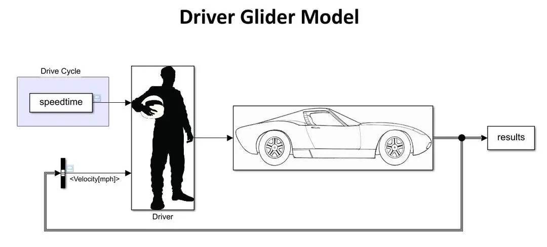
- For the Driver Glider Model, I create a Real TIme Drive Cycle on an Excel sheet(speedtime), which includes speed variation with respect to time.
- This Drive cycle (speedtime) excel sheet I import and save as numerical in MATLAB workspace. Then I use it as an input to the Driver. Using From Workspace block.

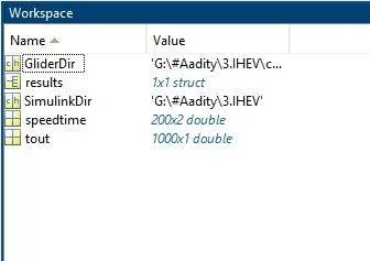
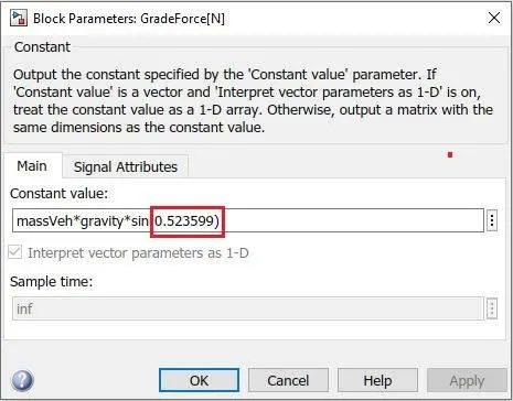
- Further to provide the Hill Climb Angle I edit in the Gradeability Force by providing the climbing angle.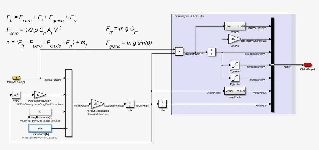
Result- 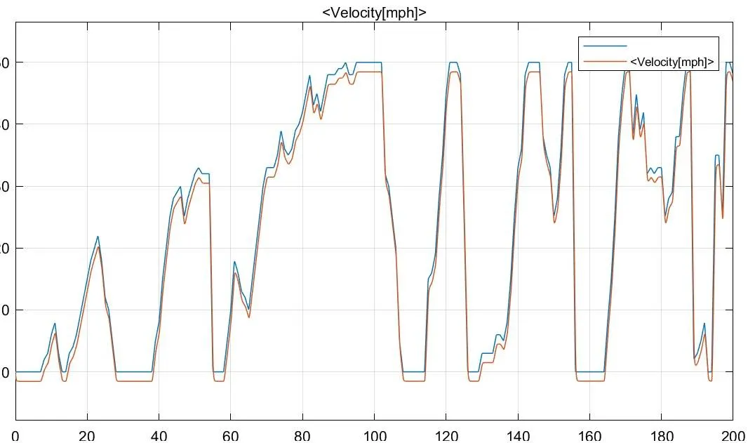
- Here from the Graph, it is shown that there is a salient difference in both the output. This is because of the difference in the input values.
- After Giving these inputs Tractive Force is Calculated acting on the vehicle including all the Parameters & Losses.
- As per the requirement, I provided the Hill climbing angle to be 30°
- Due to Hill Climbing Force more power is required for the vehicle.
- Hence on giving the acceleration vehicle requires more power so, velocity get decreases at the time of acceleration.
- While applying brakes there is no such extra power required, so the graph is shown overlapping on braking.
# Ques- 4 Model the WOT (Wide Open Throttle) response of GM EV1 car.
Compare it with the official figures for the performance of a real vehicle. Prepare a table showing variation in acceleration time with a 5% change in vehicle parameters.
Given Data :-
Drag Coefficient (Cd) = 0.19
Rolling Resistance (μrr) = 0.0048
Frontal Area (A) = 1.8 m2m2
Efficiency (ηg) = 0.95
Vehicle mass = 1400 kg
Payload mass = 140kg
- The Motor's moment of inertia is not known, however, compared to such a heavy vehicle, it will be very low, the wheels are also light as compared, so the total mass will be added by 20kg more
Total mass (m) = 1560 kg
Tire radius (r) = 0.30 m
Tmax = 140 Nm
ωc = 733 rad/s
Critical velocity (ν) = 19.8 m/s = 71.3 km/h
Assumptions-
T = Tmax until the critical velocity
above the critical velocity, the motor operates at a constant 102kW, so as it is a WOT Test 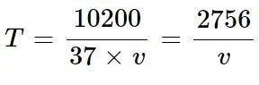
-Solve for 3 cases(Actual Parameter, 5% Increase & 5% Decrease in Vehicle Parameter)
|
Actual parameters |
5% Iecrease in Vehicle Parameters |
5% Decrease in Vehicle parameters |
|
Frontal Area (A) = 1.8 m2 Vehicle mass (m) = 1400 kg Total mass (m) = 1560 kg Tire radius (r) = 0.30 m |
Frontal Area (A) = 1.89 m2 Vehicle mass (m) = 1470 kg Total mass (m) = 1630 kg Tire radius (r) = 0.315 m |
Frontal Area (A) = 1.89 m2 Vehicle mass (m) = 1330 kg Total mass (m) = 1490 kg Tire radius (r) = 0.285 m |
The equations to be used-
Equation 1-
Equation 2-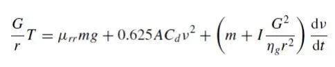
- The Max Torque of an Electric Vehicle is the function of angular speed. At low-speed Maximum Torque is constant till the motor reaches critical(ωc) speed after which Torque falls.
At Initial Acceleration assume T = Tmax
than Equation will be,
Equation 3-
# Case 1 - Considered the Actual PArameter of the vehicle GM EV1 car
Putting all the Given Data with Actual Parameter of vehicle in Equation 3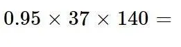
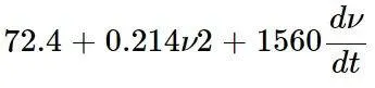
on rearranging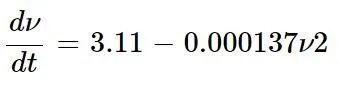
- Once the speed reached 19.8 m/s = 71.3 km/h, velocity in differential form, by putting all the values in Equation 2
for
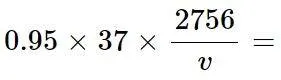
on rearranging,
- Further, these equations are put into 'Finite Difference' Form 
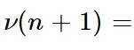

MATLAB Program- For Actual Parameter
clear all
close all
clc

% Inputs Parameter for GM EV1 Car
t = linspace(0,50,501); % 0 to 50s
vel = zeros(1,501); % 501 reading for velocity
d = zeros(1,501); % Distance travelled
dT = 0.1; % 0.1 seconf time step

% For Original Parameter of Vehicle
for n=1:500
    % Now Using Equations
    if vel(n)<19.8 %Contant Torque Till Point

        vel(n+1) = vel(n) + dT*(3.11 - (0.000137*(vel(n)^2)));

    elseif vel(n)>=19.8

        vel(n+1) = vel(n) + dT*((62.1/vel(n)) - (0.046) - (0.000137*(vel(n)^2)));
    end
    if vel(n)>35.76
        vel(n+1)=vel(n);
    end

    d(n+1) = d(n) + 0.1 * vel(n); % Distance Travelled
end

vel = vel.*3.6; % In kph

% Plotting
figure(1)
plot(t,vel);
axis([0 30 0 150]);
xlabel('Time [second]');
ylabel('velocity [kph]');
title('WOT for GM EV [Actual Parameter]')
# Case 1 - Considered the vehicle GM EV1 car increase by 5%
Putting all the Given Data with 5% increased Parameter of vehicle in Equation 3


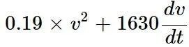
on rearranging,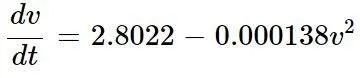
Once the speed reached 19.8 m/s = 71.3 km/h, velocity in differential form, by putting all the values in Equation 2
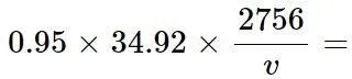
on rearranging,
- Further, these equations are put into 'Finite Difference' Form

MATLAB Program- For 5% Increased Parameter
clear all
close all
clc

% Inputs Parameter for GM EV1 Car
t = linspace(0,50,501); % 0 to 50s
vel = zeros(1,501); % 501 reading for velocity
d = zeros(1,501); % Distance travelled
dT = 0.1; % 0.1 seconf time step

% For Vehicle Parameter Increase by 5%
for n=1:500
    % Now Using Equations
    if vel(n)<19.8 %Contant Torque Till Point

        vel(n+1) = vel(n) + dT*(2.8022 - (0.000138*(vel(n)^2)));

    elseif vel(n)>=19.8

        vel(n+1) = vel(n) + dT*((56.09/vel(n)) - (0.047) - (0.000137*(vel(n)^2)));
    end
    if vel(n)>35.76
        vel(n+1)=vel(n);
    end

    d(n+1) = d(n) + 0.1 * vel(n); % Distance Travelled
end

vel = vel.*3.6; % In kph

% Plotting
figure(2)
plot(t,vel);
axis([0 30 0 150]);
xlabel('Time [second]');
ylabel('velocity [kph]');
title('WOT for GM EV [5% Increased Parameters]')
# Case 1 - Considered the vehicle GM EV1 car Decrease by 5%
Putting all the Given Data with 5% increased Parameter of vehicle in Equation 3


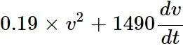
on rearranging,

Once the speed reached 19.8 m/s = 71.3 km/h, velocity in differential form, by putting all the values in Equation 2

on rearranging,

- Further, these equations are put into 'Finite Difference' Form

MATLAB Program- For 5% Decreased Parameter
clear all
close all
clc

% Inputs Parameter for GM EV1 Car
t = linspace(0,50,501); % 0 to 50s
vel = zeros(1,501); % 501 reading for velocity
d = zeros(1,501); % Distance travelled
dT = 0.1; % 0.1 seconf time step

% For Vehicle Parameter Decrease by 5%
for n=1:500
    % Now Using Equations
    if vel(n)<19.8 %Contant Torque Till Point

        vel(n+1) = vel(n) + dT*(3.398 - (0.000136*(vel(n)^2)));

    elseif vel(n)>=19.8

        vel(n+1) = vel(n) + dT*((67.82/vel(n)) - (0.047) - (0.000136*(vel(n)^2)));
    end
    if vel(n)>35.76
        vel(n+1)=vel(n);
    end

    d(n+1) = d(n) + 0.1 * vel(n); % Distance Travelled
end

vel = vel.*3.6; % In kph

% Plotting
figure(3)
plot(t,vel);
axis([0 30 0 150]);
xlabel('Time [second]');
ylabel('velocity [kph]');
title('WOT for GM EV [5% Decreased Parameters]')
Result:- Output Graph For all Three Cases
Case 1 - For Actual Parameter of the vehicle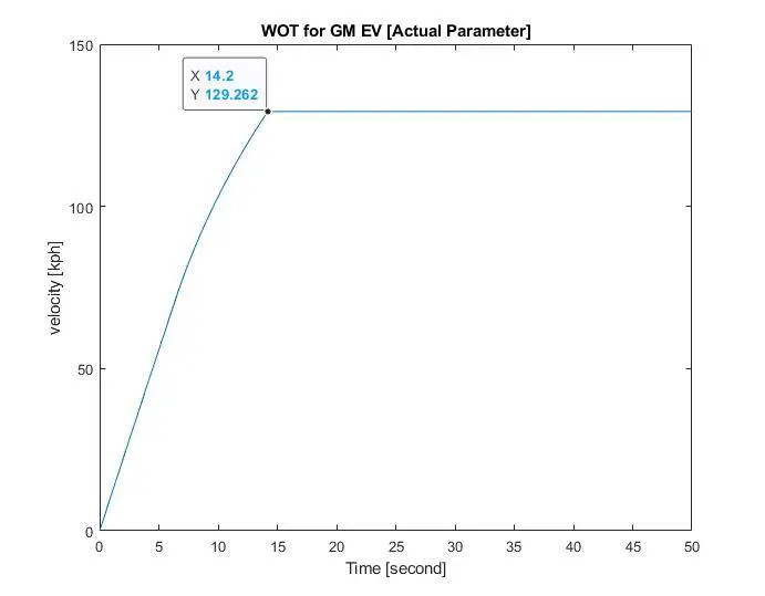
Case 1 - For 5% Increased Parameter of the vehicle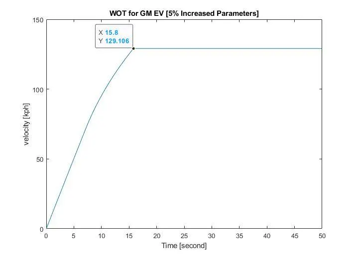
Case 1 - For 5% Decreased Parameter of the vehicle.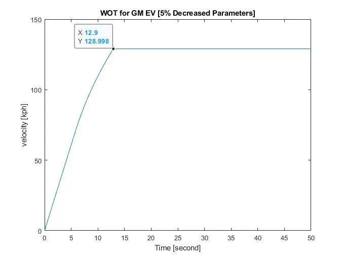
From the above results, we can conclude that
- At the Actual parameters of the vehicle, the top speed will reach after 14.2 secs.
- On Increasing the vehicle parameters by 5% then the top speed will be attained after 15.8 secs, as the vehicle parameters (weight, frontal area & the tire radius) will affect the Rolling Resistance Force, Drag Force which leads in a change of Tractive Force, vehicle experience more Tractive force on it, so more time will take to reach to a top speed.
- Same will happen when decreasing the parameters of the vehicle by 5%, then the top speed is attained more sooner in 12.9 secs, as less Tractive Force is experienced by the vehicle.
LEARNING OUTCOME
- We learn the real-time drive cycle and its effect on the vehicle.
- We learn the effect of forces on the vehicle.
- We also learn the effect of the vehicle parameter itself on its power.
- We learn the Wide Open Throttle characteristics of the GM EV1 car.