Write code to fit a linear and cubic polynomial for the Cp(Specific Heat) data. (Using Split-wise method)

AIM:- To write code to fit a linear and cubic polynomial for the Cp(Specific Heat) data.

Introduction:-

Curve Fitting:- Curve fitting is the process of constructing a curve, or mathematical function, that has the best fit to a series of data points, By Curve Fitting, we can mathematically construct the functional relationship between the observed data-set and parameter values.

Curve fitting is nothing but approximating the given function f(x) using simpler functions say polynomials, trigonometric functions, exponential functions and rational functions. However, the main difference between interpolation and Curve fitting is, in the former, the approximated curve has to pass through the given data points. Here again polynomial functions are the one which are been used widely in the applications than the other functions

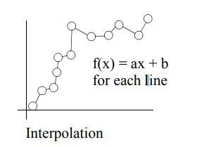
Interpolation:- (connect the data-dots)

If data is reliable, we can plot it and connect the dots. This is piece-wise, linear interpolation. This has limited use as a general function f(x). Since its really a group of small s, connecting one point to the next it doesn’t work very well for data that has built in random error (scatter)

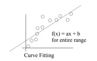
Linear curve fitting (linear regression):-

capturing the trend in the data by assigning a single function across the entire range.

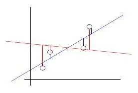
• Consider the distance between the data and points on the line.
• Add up the length of all the red and blue verticle lines.
• This is an expression of the ‘error’ between data and fitted line.
• The one line that provides a minimum error is then the ‘best’ straight line.

Given the general form of a straight line

f(x) = ax +b

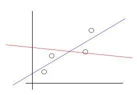
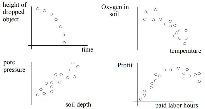
NOTE:- Straight line is not suitable for each of these cases, There are lots of functions with lots of different shapes that depend on coefficients.

Polynomial Fit:-

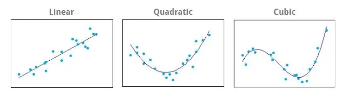
The Polynomial Fit tool in Origin can fit data with polynomial up to 9th order. Fixed intercept and apparent fit are also supported.
Consider the general form for a polynomial of order,

Quantifying error in a curve fit:-

• Positive or negative error have the same value (data point is above or below the line
• Weight greater errors more heavily (we can do both of these things by squaring the distance)

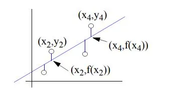
denote data values as (x, y)
denote points on the fitted line as (x, f(x))
sum the error at the four data points

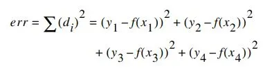
Our fit is a straight line, so now substitute f(x) = ax +b

The ‘best’ line has minimum error between line and data points This is called the least squares approach, since we minimize the square of the error.

Objective:

1. To fit a linear and cubic polynomial for the Cp data.
2. Plot the linear and cubic fit curves along with the raw data points
3. Write a code to show split-wise method

MATLAB PROGRAM:-

MATLAB code to fit a linear and cubic polynomial for the Cp data

clear all
close all
clc

%Distinguish The Data Sheet
cp_data = load('data'); % Data Sheet
tempr = cp_data(:,1);   % Temperatue
cp = cp_data(:,2);      % Specific Heat

% Curve Fit 

% cp1 = a*temp + b | Linear polynomial
co_effs1 = polyfit(tempr, cp,1);
predicted_cp1 = polyval(co_effs1,tempr);

% cp2 = a*temp^3 + b*temp^2 + c*temp + d | Cubic polynomial
co_effs2 = polyfit(tempr, cp,3);
predicted_cp2 = polyval(co_effs2,tempr); 


%Compare original data to fitted data of 1st order & 3rd order
hold on
plot(tempr,cp,'linewidth',2,'color','g')            % original data set
plot(tempr,predicted_cp1,'linewidth',2,'color','m') % First order Curve-fit
plot(tempr,predicted_cp2,'linewidth',2,'color','b') % Second order Curve-fit
xlabel('Temperature [k]')
ylabel('Specific Heat [KJ/Kmol-k]')
legend('Original data' , 'First order Curve-fit' , 'Second order Curve-fit')
title('Specific Heat v/s Temperature [For Linear & Cubic Curve Fitting]') 

% To Calculate Quality of fit For Linear Polynomial(First Order)
SSR_1 = sum((predicted_cp1 - mean(cp)).^2);         %sum of squares regression
SSE_1 = sum((predicted_cp1 - cp).^2);               %sum of squares error
SST_1 = SSR_1 + SSE_1;                              %sum of squares total

%Quality of fit R-squared(R_sq) = SSR/SST 
%For Linear Polynomial(first Order)
R_sq_1 = (SSR_1/SST_1)


% To Calculate Quality of fit For Cubic Polynomial(Second Order)
SSR_2 = sum((predicted_cp2 - mean(cp)).^2);       %sum of squares regression
SSE_2 = sum((cp - predicted_cp2).^2);             %sum of squares error
SST_2 = SSR_2 + SSE_2;                            %sum of squares total
 
%Quality of fit R-squared(R_sq) = SSR/SST 
%For Cubic Polynomial(Second Order)
R_sq_2 = (SSR_2/SST_2)

MATLAB Coding using split-wise method

clear all
close all
clc

%Distinguish The Data Sheet
cp_data = load('data');
tempr = cp_data(:,1);
cp = cp_data(:,2);

% Curve Fit 

%using splitwise Method
a = 1;
b = 3200/4;

%Using For Loop

for i = 1:4
   temp(:,i) = tempr(a:b);
   
   
% cp1 = a*temp + b | Linear Polynomial
co_effs1= polyfit(tempr(a:b), cp(a:b),1);
predicted_cp1 = polyval(co_effs1,tempr(a:b));


 % For Quality of Fit  | SST = SSR + SSE
  
SSR = sum((predicted_cp1 - mean(cp)).^2);    %sum of sq of regression
SSE = sum((cp(a:b) - predicted_cp1).^2);     %sum of sq error
SST = SSR + SSE;                    

%Goodness OF Fitting | R_sq = (SSR/SST)
R_sq(i) = (SSR/SST);


a = b + 1;
b = b + 3200/4;


  predicted_cp1_new(:,i)= predicted_cp1;
  
 
end 

 %plot  
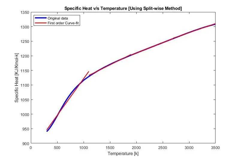
  plot(tempr,cp,'linewidth',3,'color','b')
  hold on
  plot(temp(:,1),predicted_cp1_new(:,1),'linewidth',2,'color','r')
  plot(temp(:,2),predicted_cp1_new(:,2),'linewidth',2,'color','r')
  plot(temp(:,3),predicted_cp1_new(:,3),'linewidth',2,'color','r')
  plot(temp(:,4),predicted_cp1_new(:,4),'linewidth',2,'color','r')
  xlabel('Temperature [k]')
  ylabel('Specific Heat [KJ/Kmol-k]')
  legend('Original data' , 'First order Curve-fit')
  title('Specific Heat v/s Temperature [Using Split-wise Method]')

  
%Quality of fit R-squared(R_sq) = SSR/SST 
%For Linear Polynomial(first Order) using Split-wise method
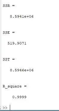
R_square = mean(R_sq(i))

Procedure:

Using Split-wise Method

Step 1-. Firstly I start with loading the provided data sheet{Temperature(tempr) & Specific heat(cp)} using Load command and Distinguish the data into Temperature and specific-Heat array.

Step 2- Now, I use Split-wise method for fitting the curve.
For that I use two variable a,b and provide the value from 1 & 800, wich will be used for the for loop, and use ‘i’ variable from 1:4, and put the value of tempr(a:b) into new variable temp

Step 4- Now, by using Polyfit, it returns the coefficients for a polynomial p(tempr) of degree 1 that is a best fit (in a least-squares sense) for the data in (cp). Now by using Polyval command, evaluates the polynomial at each point in tempr. Form here we, get the Predicted Specific heat (predicted_cp1).

Step 5- For the Quality of Fit, i Calculate the SSR,SSE,SST and the values in variable R_sq(i) to get the Values of Goodness of fit.

Step 6- In this Step, to run the loop till the exceeding value till 3200. I put the new value for a=b+1 and b=b+800. it will run the loop till it will reach its final value for temperature.

Step 7- Now, in this I store the values Predicted specific heat(predicted_cp) into new Variable array vpredicted_cp_new, so that it can be used to plot all the split curve into Graph

Step 8 - Now I plot the comparison Graph of original data_sheet and Linear fir curve after splitting. Use x-label as temperature and y-label as Specific Heat. And tittle the Graph as Specific Heat v/s Temperature (Using Split-wise Method)

Step 9- Lastly I calculate the goodness of fit R_square by putting the value of variable R_sq(i) and mean of this value

Parameters used to measure the fitness characteristics for both the curves:-

Upon finding a curve which satisfy the data there are 4 quantities which help us measure the goodness of fit criteria or how well the equation is a representing the data-points. There are,

The sum of Square due to Error (SSE)
R-square
Adjusted R-square
Root mean Squared Error (RMSE)

R-square:- Quantity that measures how successful the fit is in explaining the variation of the data.It is a relative measure and takes values ranging from 0 to 1. R-Square is the correlation between the response values & the coefficient of multiple determination.
The value of R-square can be calculated using the formula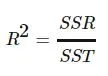

SSR = The sum of squares due to regression, or SSR. It is the sum of the differences between the predicted value and the mean of the dependent variable.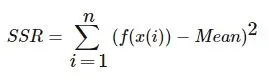

SSE = The sum of squares error, or SSE. The error is the difference between the observed value and the predicted value.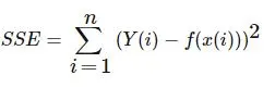

SST = The sum of squares total, denoted SST, is the squared differences between the observed dependent variable and its mean.

Results:-

• Plot the linear and cubic fit curves along with the raw data points.

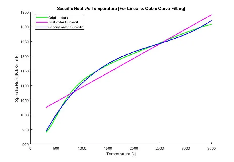
• Plot the linear fit curves along with the raw data points using split-wise method

Goodness Of Fit

For linar polynomial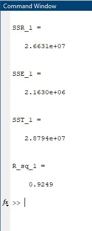

For Cubic Polynomial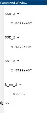


Goodness of Fit Using Split-wise Method

Based on the research, answer for following questions are:

1. How to make a curve fit perfectly?
   Ans:- to make a fit there are no. method can be used, like
   -Split-Wise Method
   -Different Polynomial Order
   -One Polynomial for one Temperature Range and Different Polynomial Oreder for Different Temperature Range.
   
   
2. How to get the best fit?
   Ans:- Upon finding a curve which satisfy the data there are 4 quantities which help us measure the goodness of fit.
   The sum of Square due to Error (SSE)
   R-square
   Adjusted R-square
   Root mean Squared Error (RMSE)
3. What could be done to improve the cubic fit?
   Ans:- We can use use the Split-Wise Method and Fitted the curve by spliting the curve over the actual data.
   we can make a program which ask the user of number of split, so that best fit after split can be made.