Solve the Second Order ODE(Ordinary Differential Equation) Using MATLAb

AIM:- To Write a program in MATLAB to Solve the Second Order ODE(Ordinary Differential Equation).

Introduction:- In mathematics, an ordinary differential equation (ODE) is a differential equation containing one or more functions of one independent variable and the derivatives of those functions.

Example;- in order is to solve an ODE, determine what function or functions satisfy the equation,

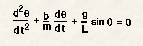
Above, is the Second Order order Ordinary Differential Equation that represents, the equation of motion of a simple pendulum with damping,

(The way the pendulum moves & the position of the "ball" w.r.t time).

In the above equation,

g = gravity in m/s2,

L = length of the pendulum in m,

m = mass of the ball in kg,

b=damping coefficient.

Objective:

1. To write a program that solves the following ODE For Simple Pendulum.
2. Write a program in MATLAB that will simulate the pendulum motion.

Procedure:

Step 1- Firstly we need to provide the values for

L=1 metre,

m=1 kg,

b=0.05.

g=9.81 m/s2.

And simulate the motion between 0-20 sec,

for angular displacement=0,

angular velocity=3 rad/sec at time t=0.

Step 2- Using Linspace to get 500 values, for time span b/w 0-20 sec.

Step 3- Now, to solve and ODE, I am using the inbuilt solver ODE45 to solve for Angular Displacement & Angular Velocity as results.
For that I am Scripting a different function {ode_func(t,theta,b,g,l,m)},

which represents how our ODE function is define.

theta1 = theta(1);

theta2 = theta(2);

dtheta1_dt = theta2;

dtheta2_dt = -(b/m)*theta2 - (g/l)*sin(theta1);

dtheta_dt = [dtheta1_dt; dtheta2_dt];

Where,

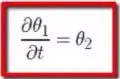is First ODE.

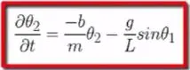is Second ODE.

Step 4- Now this function on computing with the Second order ODE Program will give the integration time & results
Since, we are solving for 2 ODE’s the results will be a column vector which consist of 2 column, the first one refers to Angular Displacement & the Second one refers to Angular Velocity.

Step 5- Now, Plotting these results on Graph.
Figure-1

Step 6- Now I am scripting to simulate the pendulum motion on Graph by giving the Coordinate points for ball, using ‘for loop’ command

x0 = 0;

y0 = 0;

x1 = l*sin(results(i,1));

y1 = -l*cos(results(i,1));

Step 7- In last Step, to get an output as Video of Graphical representation, i type the codes for the Graphical representation to plot the all points on x y coordinates, add use 'pause command' to pause the graph for a particular time period and use 'M(ct)' to capture the current frame every time for the 'for loops’ End the 'for loop' followed by code 'ct=ct+1' for increment the frame every time when the for loop run.

And Lastly to make a video "movie' command is used, where, 'AVI' format is used in VideoWriter to save file in AVI format, and 'writeVideo' command is used to write the plots in video format. and close' is used to close and save the video file on computer.

MATLAB PROGRAM:-

• Matlab code to get the Graphical representation of Curve b/w (Angular Velocity, Angular Displacement) with respect to Time.

%MATLAB Programme to solve equation of motion for simple pendulum with damping

clear all 
close all
clc

%inputs
b=0.05; %Damping - (Ns/m)
g=9.81; % Gravity - (m/s^2)
l=1;    % Length Of String- (m)
m=1;    % Mass - (kg)

%initial Condition
theta_0 = [0;3]; % [Angular_Displacement(0); Angular_Velocity(3 ra/sec)]


% time points
t_span = linspace(0,20,500); %Time_Span (0-20Sec)


%solve ODE
[t, results] = ode45(@(t,theta) ode_func(t,theta,b,g,l,m),t_span, theta_0);


figure(1)
hold on
plot(t,results(:,1))
hold on
plot(t,results(:,2))
hold off
ylabel('Velocity(m/s^2), Displacement(m/s)')
xlabel('Time(s)')


%Pendulum Animation
ct=1;
for i= 1:length(results(:,1))
    
        %Coordinates
x0 = 0;
y0 = 0;

x1 = l*sin(results(i,1));
y1 = -l*cos(results(i,1));

    %Outputs- Graphical Representation & Animation

figure(2)
plot([-2 2],[0 0],'linewidth',10)

hold on
line([x0 x1],[y0 y1],'linewidth',3,'color','m')
axis([-2 2 -2 0])
hold on
plot(x1, y1,'O','markers',15,'linewidth',20,'color','g')
title('Simulation for Damped pendulum motion','fontsize',15)
hold off

pause(0.01);
M(ct) = getframe(gcf);
ct=ct+1;

end

hold on
%Video Animation
movie(M)
videofile = VideoWriter('Pendulum animation.avi','Uncompressed AVI');
open(videofile)
writeVideo(videofile,M)
close(videofile)

• Matlab Coding to create the Function named ode_func as follows:-

function [dtheta_dt] = ode_func(t,theta,b,g,l,m)

theta1 = theta(1);
theta2 = theta(2);
dtheta1_dt = theta2;
dtheta2_dt = -(b/m)*theta2 - (g/l)*sin(theta1);
dtheta_dt = [dtheta1_dt; dtheta2_dt];
end

Results:-

• Below Figure-1 is the Graphical representation showing the Curve b/w (Angular Velocity, Angular Displacement) with respect to Time.

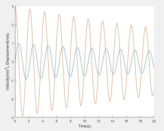
Figure-1

• Below is the link to support my presentation (video for Simulation of the pendulum motion)

https://drive.google.com/file/d/1Zl6IEskn8-UiZVsuy-nQGJoE6H5VsyPs/view?usp=sharing