MATLAB code to optimize the stalagmite function and find the Global Maxima of the function using Genetic Algorithm
AIM:- Write a code in MATLAB to optimize the stalagmite function and find the Global Maxima of the function.
Introduction:- Genetic Algorithm (GA) is a search-based optimization technique based on the principles of Genetics and Natural Selection. It is frequently used to find optimal or near-optimal solutions to difficult problems which otherwise would take a lifetime to solve. It is frequently used to solve optimization problems, in research, and in machine learning
Theory:-
Optimization:- Optimization is the process of making something better. In any process, we have a set of inputs and a set of outputs as shown in the following figure.
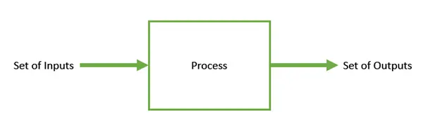
Optimization refers to finding the values of inputs in such a way that we get the “best” output values. The definition of “best” varies from problem to problem, but in mathematical terms, it refers to maximizing or minimizing one or more objective functions, by varying the input parameters.
The set of all possible solutions or values which the inputs can take make up the search space. In this search space, lies a point or a set of points which gives the optimal solution. The aim of optimization is to find that point or set of points in the search space.
Genetic Algorithm- Nature has always been a great source of inspiration to all mankind. Genetic Algorithms (GAs) are search based algorithms based on the concepts of natural selection and genetics. These are intelligent exploitation of random search provided with historical data to direct the search into the region of better performance in solution space. They are commonly used to generate high-quality solutions for optimization problems and search problems.
In GAs, we have a pool or a population of possible solutions to the given problem. These solutions then undergo recombination and mutation (like in natural genetics), producing new children, and the process is repeated over various generations. Each individual (or candidate solution) is assigned a fitness value (based on its objective function value) and the fitter individuals are given a higher chance to mate and yield more “fitter” individuals. This is in line with the Darwinian Theory of “Survival of the Fittest”.
In this way we keep “evolving” better individuals or solutions over generations, till we reach a stopping criterion.
Genetic Algorithms are sufficiently randomized in nature, but they perform much better than random local search (in which we just try various random solutions, keeping track of the best so far), as they exploit historical information as well.
The genetic algorithm uses three main types of rules at each step to create the next generation from the current population:
- Selection rulesselect the individuals, called parents, that contribute to the population at the next generation.
- Crossover rulescombine two parents to form children for the next generation.
- Mutation rulesapply random changes to individual parents to form children.
How the Genetic Algorithm Works
Outline of the Algorithm
The following outline summarizes how the genetic algorithm works:
- The algorithm begins by creating a random initial population.
- The algorithm then creates a sequence of new populations. At each step, the algorithm uses the individuals in the current generation create the next population. To create the new population, the algorithm performs the following steps:
- Scores each member of the current population by computing its fitness value. These values are called the raw fitness scores.
- Scales the raw fitness scores to convert them into a more usable range of values. These scaled values are called expectation values.
- Selects members, called parents, based on their expectation.
- Some of the individuals in the current population that have lower fitness are chosen as elite. These elite individuals are passed to the next population.
- Produces children from the parents. Children are produced either by making random changes to a single parent—mutation—or by combining the vector entries of a pair of parents—
- Replaces the current population with the children to form the next generation.
- The algorithm stops when one of the stopping criteria is met.
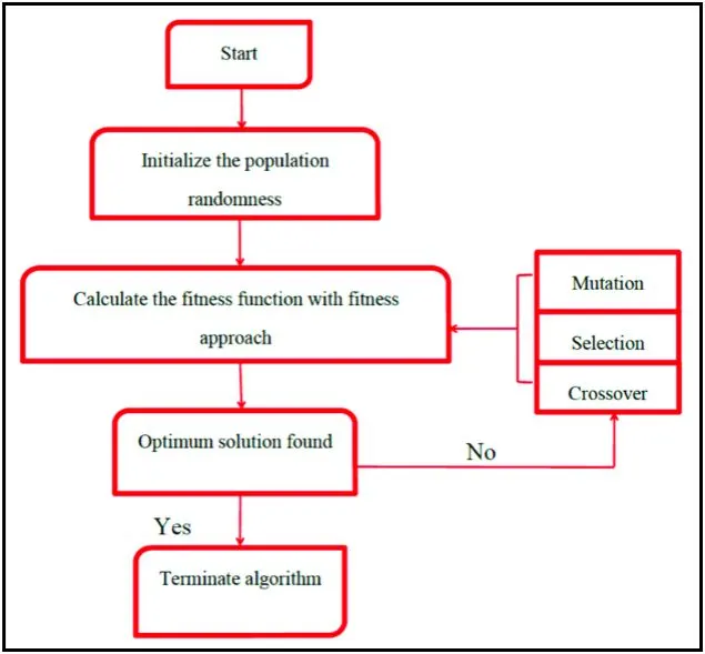
Operators of Genetic Algorithms
Once the initial generation is created, the algorithm evolve the generation using following operators –
1) Selection Operator: The idea is to give preference to the individuals with good fitness scores and allow them to pass there genes to the successive generations.
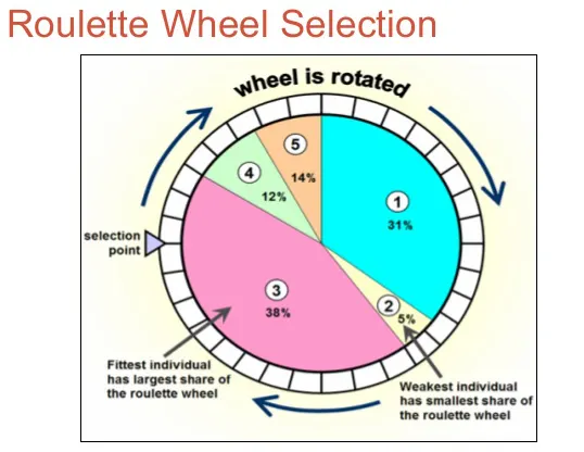
In a roulette wheel selection, the circular wheel is divided with respect to the Fitter individual. A fixed point is chosen on the wheel circumference as shown and the wheel is rotated. The region of the wheel which comes in front of the fixed point is chosen as the parent. For the second parent, the same process is repeated.
In this way Fitter individual have a higher chance of mating and propagating their feature to the next generation.
2) Crossover Operator: This represents mating between individuals. Two individuals are selected using selection operator and crossover sites are chosen randomly. Then the genes at these crossover sites are exchanged thus creating a completely new individual (offspring).
For example –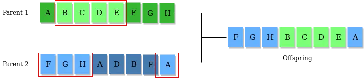
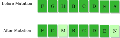
3) Mutation Operator: The key idea is to maintain the diversity from one generation of population of chromosomes to the next.
If mutation is not performed, the chromosomes will become to similar to each other,convergence takes place soon and results in local minima
example- Insert random genes in offspring, here random genes are inserted to maintain the diversity.
Parameters used in Genetic Algorithms
Fitness Function- A fitness function is a particular type of objective function that is used to summaries, as a single figure of merit, how close a given design solution is to achieving the set aims. Fitness functions are used in Genetic Programming and Genetic Algorithm to guide simulations towards optimal design solutions
Objective:
- To Understand the concept of genetic algorithm
- To Understand the syntax “ga” in MATLAB
- To find the Global Maxima of the stalagmite function in MATLAB
MATLAB PROGRAM:-
- MATLAB code to optimize the stalagmite function and find the Global Maxima of the function
%% clean all
clear all; close all; clc

%% Defining Our Search Space
x = linspace(0,0.6,150);
y = linspace(0,0.6,150);
num_cases = 50                                            % no of itration

%% Creating a 2Dimensional mesh
[xx ,yy] = meshgrid(x,y);

%% Evaluating the Stalagmite Function
for i = 1:length(xx)
    for j = 1:length(yy)
        input_vector(1)=xx(i,j);
        input_vector(2)=yy(i,j);
        input_vector=[input_vector(1),input_vector(2)];
        GA(i,j) = stalagmite(input_vector);               %Calling the Createdc Function

    end
end


%% Study-1 | Statistical Behaviour | In Unbounded condition

tic                                                       %tic_toc command for calculating the itration time
for i = 1:num_cases
        [input, GA_opt(i)] = ga(@stalagmite,2);
        xopt(i) = input(1);
        yopt(i) = input(2);
end

study_1_time = toc

%Plotting the Graph
figure(1)
subplot(2,1,1)
hold on
surfc(x,y,-GA)
shading interp
plot3(xopt,yopt,-GA_opt,'marker','o','markersize',5,'markerfacecolor','r')
title('Unbounded inputs')
subplot(2,1,2)
plot(-GA_opt)
xlabel('Iteration')
ylabel('Function Minium')


%% Study-2 | Statistical behaviour - with upper & lower bounds

tic                                                      %tic_toc command for calculating the itration time
for i = 1:num_cases
    [input, GA_opt(i)] = ga(@stalagmite,2,[],[],[],[],[0;0],[1;1]);
        xopt(i) = input(1);
        yopt(i) = input(2);
end
study_2_time = toc

%Plotting the Graph
figure(2)
subplot(2,1,1)
hold on
surfc(x,y,-GA)
shading interp
plot3(xopt,yopt,-GA_opt,'marker','o','markersize',5,'markerfacecolor','r')
title('Bounded inputs')
subplot(2,1,2)
plot(-GA_opt)
xlabel('Iteration')
ylabel('Function Minium')


%% Study-3 | Increasing GA Iterations

options = optimoptions('ga');                              %Calculating the optimum solution for 'ga' and save in options(variable)
options = optimoptions(options,'PopulationSize',240);      %increasing the size of population

tic                                                        %tic_toc command for calculating the itration time
for i = 1:num_cases
    [input, GA_opt(i)] = ga(@stalagmite,2,[],[],[],[],[0;0],[1;1],[],[],options);
        xopt(i) = input(1);
        yopt(i) = input(2);
end
study_3_time = toc

%Plotting the Graph
figure(3)
subplot(2,1,1)
hold on
surfc(x,y,-GA)
shading interp
plot3(xopt,yopt,-GA_opt,'marker','o','markersize',5,'markerfacecolor','r')
title('Bounded inputs')
subplot(2,1,2)
plot(-GA_opt)
xlabel('Iteration')
ylabel('Function Minium')
- MATLAB program for the function.
function [GA] = stalagmite(input_vector)

x=input_vector(1);
y=input_vector(2);


term1 = pi*5.1*x;
term2 = pi*5.1*y;
term3 = ((x-0.0667)^2/0.64);
term4 = ((y-0.0667)^2/0.64);
term5 = (-4)*log(2);

xf1 = (sin(term1 + 0.5)).^6;

yf1 = (sin(term2 + 0.5)).^6;

xf2 = exp(term5*term3);

yf2 = exp(term5*term4);


GA=-(xf1*yf1*xf2*yf2);

end
Procedure:
Step 1- Start with usual Clear and closing command to clear memory. than defines the search space with 2 variable x & y. For that, creates 1-dimensional array for x,y & use linspace command to provide 150 value between 0 to 0.6.
After that I creates 2-dimensional array based on our 1-dimension array
Step 2- In next step, by using ‘for loop’, I define the Than I am creating an array called input_vector1, input_vector2 (row vectors) for each value of x,y and save these value in
input_vector.
Step 3- Now, to calculate maxima, I am typing a new function in
@stalagmite, by using the below formula-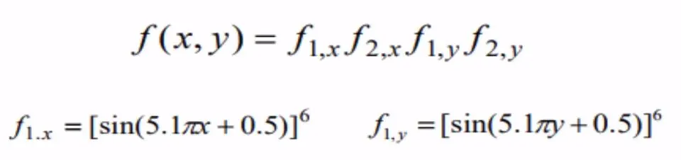
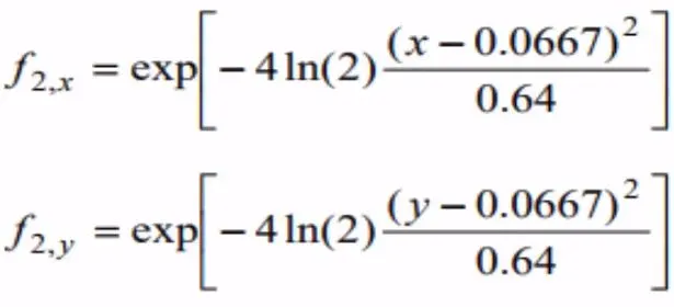
And stored its value in ‘GA’ Function.
Than this function, is called in for loop & passing the number of variable as input. So, that ‘for loop’ will generate the data for plot.
NOTE:- Genetic Algorithm is actually based on Random sample, means it will start with random sample of inputs & based on inputs we evaluate the function, than comes on some natural selection & do mates & also cross-over & than creates a new generation which is better.”But every time we run ‘ga’ code we get different results, which is not useful.
’To get beneficial results i am doing some changes in inputs and check compare the results.
I am doing three Studies to get desired output(maxima)
Step 4-
Study1- Statistical Behaviour
After creating x,y variable(input variable),
as it does not define the search space for ‘ga’, ‘ga’ does not know its actual space and the value for x,y go beyond or below to 0.6 or 0.
For that I use num_cases=50, means I am going to run it 50 times.
Sub-Step 1- I use ‘for loop’ and run the code from 1 to 50 times.
After that I call ga & use the new function which I created @stalagmite, pass 2 variable as input and store the output in GA_opt.
And than I store the value of ‘x &y’ in ‘xopt & yopt’
Sub-Step 2- Now to visualize my output, i use surface command(surfc), shading command(shading interp) is used to get smooth plot(without grid lines). in new figure window(figure1), I also use tic-toc command to calculate the time taken for evaluation. I use subplot command for multiple plotting,
1st plot to show stalagmite function, and plotting the minimum value that ‘ga’ trying to predict, over 50 studies.
2nd plot for showing the number of iteration at x-axis and during each iteration value changes which represents as Function maxima on y-axis.
Results for study-1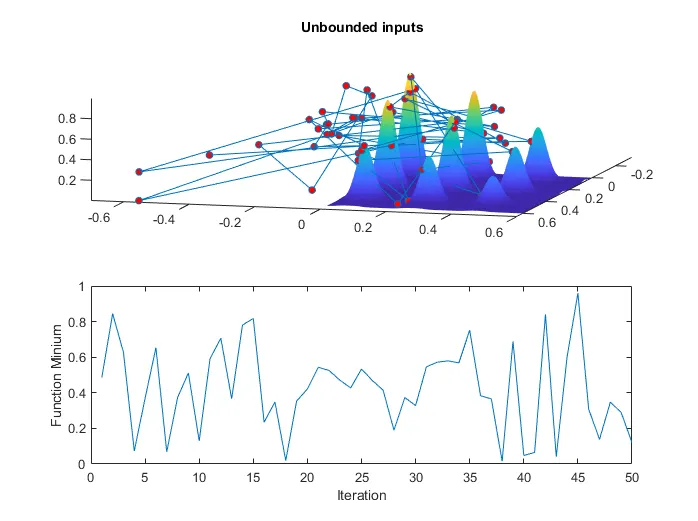
- Here on plotting stalagmite function, I am plotting the minimum value that ‘ga’ predicts, which is all over the place on graph, “it happens due to random sample during each iteration the value changes.
- Also in command window, we can observe the time taken for iteration is (study_1_time = 4.6723)sec
Step 5-
Study2- Statistical Behaviour(with upper & lower bound)
Sub-Step 1- In this study, I setup the bound condition for the variables x&y, as it is going above & below the 0 & 0.6.
By using syntax ‘ga’ I am giving x&y the upper limit and lower limit to 0 to 1. I a doing so, because in previous study, it was observed from the graph that the optimum output lies all over the graph, so make it more clear and optimum, I am applying the boundary condition.
Results for study-2 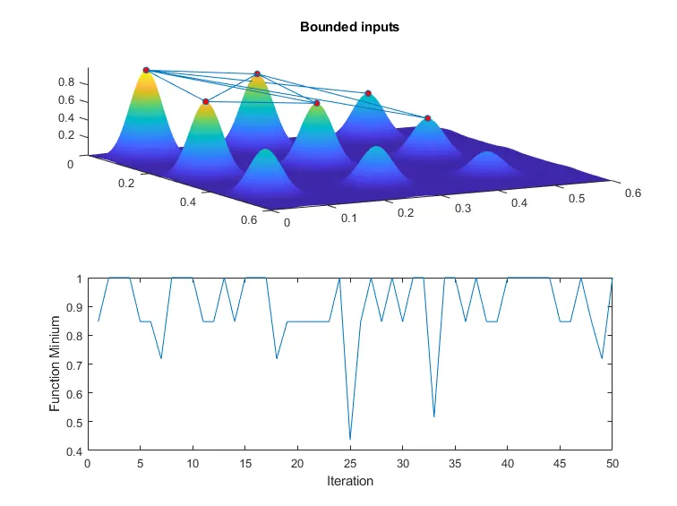
- Here from the graph, it is observed that the function predict minimum points is between 3peaks, it is much clear than Styudy-1
- If look at graph y-axis minimum values lies between 0.4 & 0.6, it is much accurate, but still not clear.
- Also , we can observe the time taken for iteration is (study_2_time=6.1982)sec, which is more than the study-1
Study3 - Increasing GA Iterations
Sub-Step 1- In addition with specifying bounds, I am also increasing initial population size. If population size is too small, we cannot find the global maxima, but we can find only local maxmia, which happens in study2.
Following the same procedure as in study-2, and increase the population size to 240 and applying the constraint ‘optimoptions’ and save its values in variable ‘options’ to allow the ga to predict the optimum solution from 240 population size.
And plot graph for visual result
Results for study-3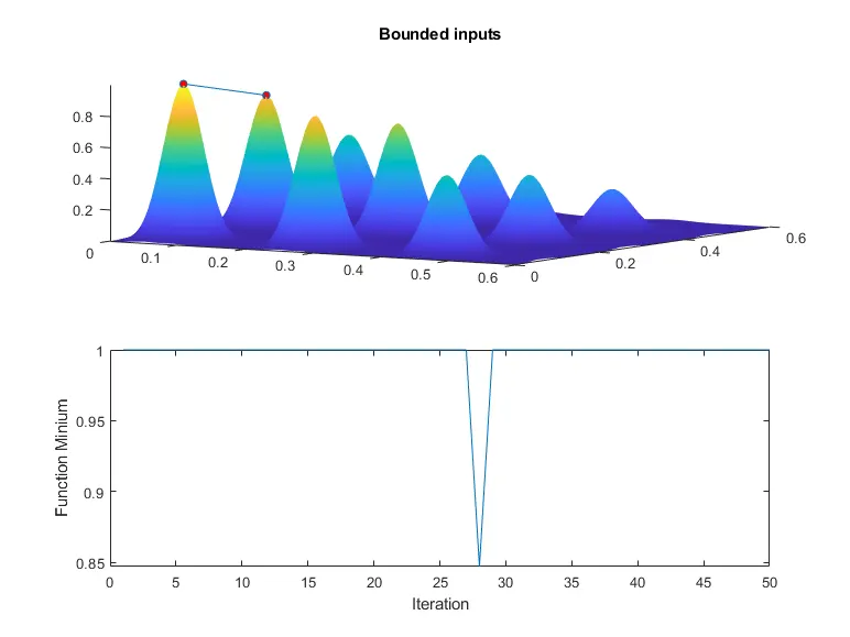
- Here from subblot-1, it shows maxima only lies around 1peak
- Maxima lies at around the value 0.85 that ga predicts
- In this study it giving the optimum value, on increasing the number Of iteration and applying constraints, but it has its drawbacks, as ga slows down as it have more number of samples, to process and evaluate them for the function.
- It takes (study_3_time =22.5917)sec, which is 6times higher than the study1.
Based on the research, answer for following questions are;
Stopping criteria-
When there has been no improvement in the population for X iterations.
- When we reach an absolute number of generations.
- When the objective function value has reached a certain pre-defined value.
Syntax for ga- ga(@stalagmite,2,[ ],[ ],[ ],[ ],[0;0],[1;1],[ ],[ ],options)
ga(fun,nvars,A,b,Aeq,beq,lb,ub,nonlcon,options)
ga - To find the minimum of function using Genetic Algorithm
fun - finds a local minimum to function
nvars - number of variables.
A - Linear Inequality Constraints,specified as a real matrix
b - Linear Inequality Constraints,specified as a real vector
Aeq - Linear equality Constraints,specified as a real matrix
beq - Linear equality Constraints,specified as a real matrix
lb - Lower Bound
ub- Upper Bound
nonlcon - Nonlinear Constraints, specified as function handle
options- Optimization options, specified as the output
Significance of running multiple iterations -
We do Multiple iteration is to get the Global maxima in desired range. The main motive of doing so is to get the only 1 desired optimum output which is required for given problem.
Links and references:-
https://en.wikipedia.org/wiki/Genetic_algorithm#Termination
https://www.tutorialspoint.com/genetic_algorithms/genetic_algorithms_quick_guide.htm
https://in.mathworks.com/help/gads/what-is-the-genetic-algorithm.html
https://drive.google.com/drive/folders/1Qj3tR9HsD4SZHvPaGKYmakpXEqv5Kb6e