Week 9 - PCB Thermal Simulation

Aim: To perform an icepak simulation for the given PCB for:

i. Conduction only for the Board Outline

ii. forced convection analysis for the entire model

iii. Joule/trace heating for the given model

Procedure:

Step 1:

• Unpack the A11.tzr
• Import the ECAD file under the choose type menu and Ansoft Neutral ANF. (A1.anf)
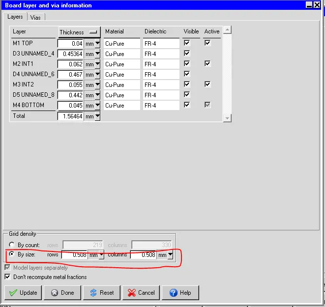
• Update the layer details as given in the problem and also specify the grid density as 0.508 mm x 0.508 mm as shown in Fig. 1

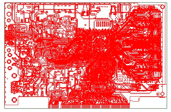
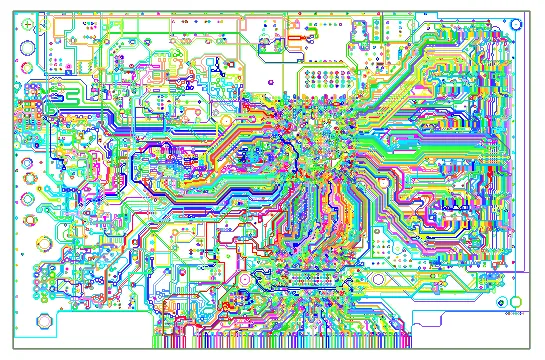
The traces in single colour, colour by trace and colour by layers are shown in figures below respectively.

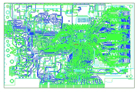
Step 2: The problem is solved for conduction only

• Keep only the PCB and make all other objects inactive. Also, autoscale the cabinet
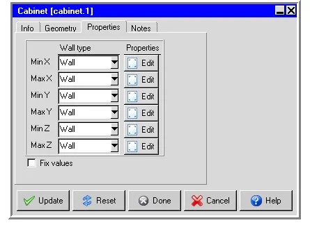
• The Min Z and Max are set for the boundry conditions of 20^oC and a heat flux of 20000 W/m²
• The other sides are insulated as given in the model.
• An initial mesh is created with the Max element Size as given min the problem. The volume mesh of the board is shown in fig. 2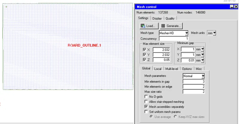Fig. 2. Volume mesh of the board.

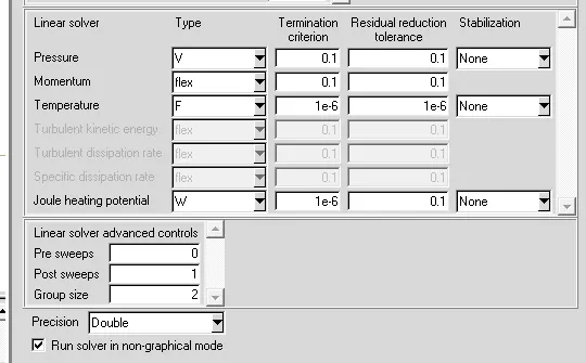
• The problem is setup only for temperature and solved for steady state conditions. under advanced settings, the temperature type is selected as F, and the terminatin criterion and residual reduction tolerance is set for 1e-6.
• 

Step 3:

• After the convergence, the results are plotted for temperature and thermal conductivity in z direction in fig. 3 and 4 respectively.
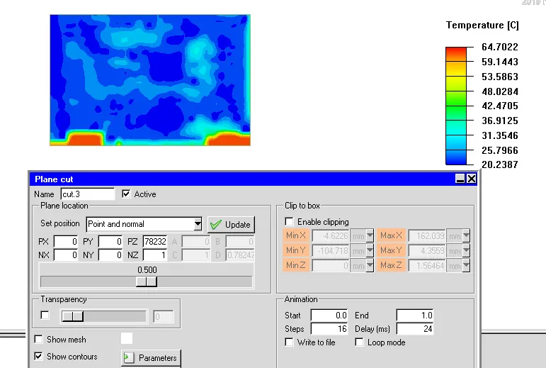• Fig. 3. Temperature contour in the board

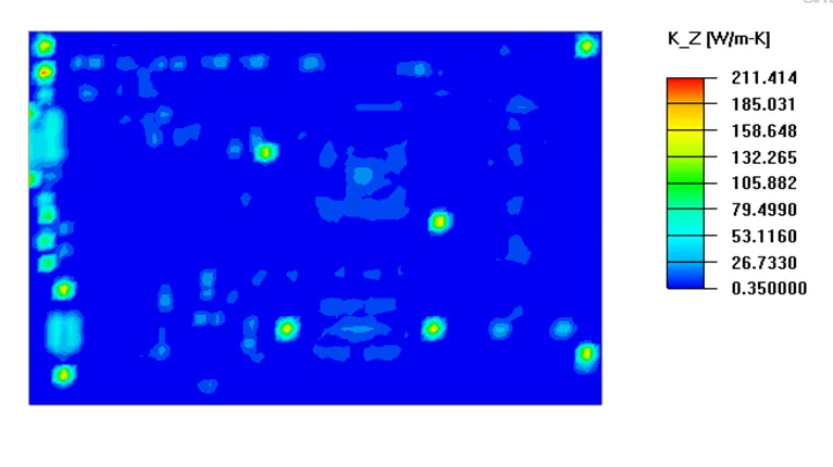Fig. 4. K_Z Thermal conductivity in Z direction in the board.

Step 4: The problem is solved for forced convection

• The inactive components are made active. The cabinet is autoscaled to cover all the components.
• The Max X is given an opening boundary condition and X velocity of -1.5 m/s specified.

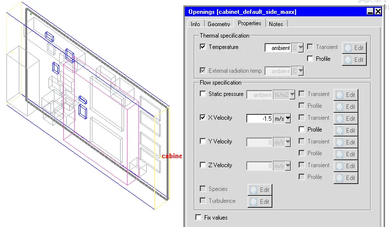
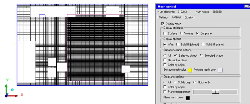
• The domain is meshed again.
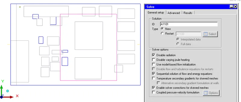
• The problem is solved for velocity and temperature with zero equation turbulence model under steady state conditions. The ambient temperature is assumed to be 20^oC and is solved with double precision.
• 
• After achieving the required convergence, the results are plotted.
• The temperature contour at the given location is shown in fig. 5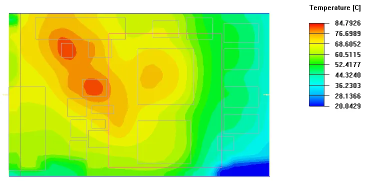Fig. 5 Temperature contour at given value of Px, Py and Pz

Similarly, the thermal conductivity in Z direction is shown in Fig. 6

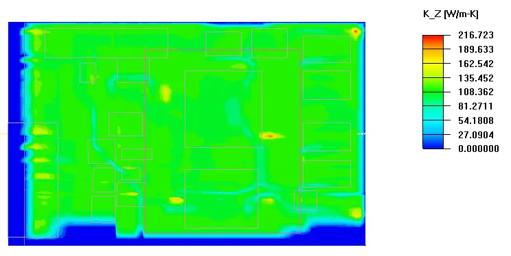Fig. 6 K_Z thermal conductivity

Step 5: Joule / Trace heating

Since PCB traces generates heat (as they have electrical resistances), understanding of the temperature distribution is very important. Hence it needs to be modeled.

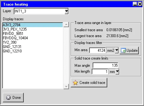
• In the geometry of the PCB, under the 'Model trace heating option, the INT1_3 layer is selected and the minimum area is entered as 4124 mm²
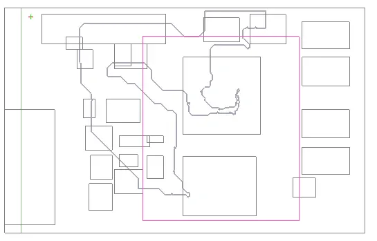
• The maximum angle and the minimum length is set to 135o and 1.0 mm respectively and a solid trace is created.
• 
• The created solid trace is shown below.
• 
• Creating two sources as specified in the problem is shown below
• 
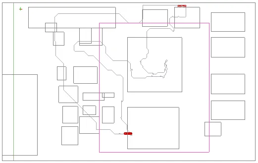
• For the source 1, a Current of 20 Amp is given and for source 2, a voltage of 0 V is given. This sets up the voltage potential and the current flows in the trace.

The boundary conditions are same for the Max X as specified in the previous case. The mesh is generated by specifying the Max X, Y and Z element size as 9.5, 7 and 0.75 mm respectively.

The volume mesh of the trace is shown below.

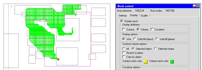
Now, the problem is run for the same conditions. For stabilization of Temperature and Joule heating, BCGSTAB is chosen.

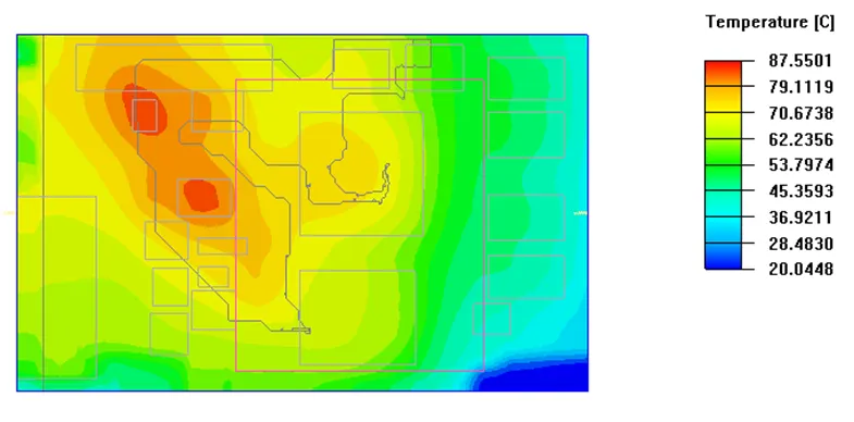
After the convergence, the temperture contour and Electric Potential are plotted for the trace.

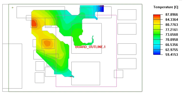
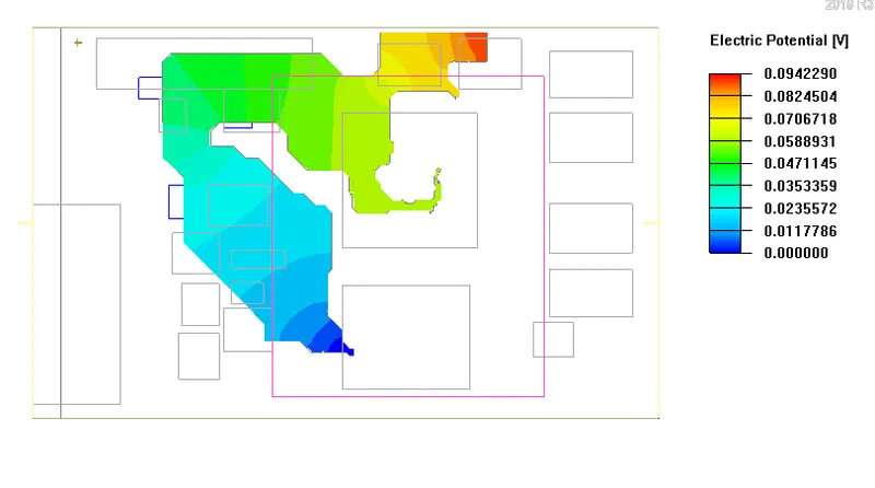
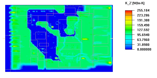
The temperature on the PCB and the thermal conductivity in Z direction are also plotted.

Conclusion:

In this challenge, the unpacking of the the PCB and importing the traces on the PCBare learnt. The traces are viewed based on the colour, layer or trace are seen. Viewing of the metal fractions in each layer are seen.

The simulation on PCB is studied for the following three cases.

i. by considering only the board which genertes around 20000 W/m² and temperature of 20^oC. The maximum temperature in the board is found to be 64^oC.

ii. Considering all the components, and with the flow velocity of -1.5 m/s in X direction, the maximum temperature is found to be 85.39^oC.

iii. For the Joule/trace heating, the maximum temperature is found to be 87.5^oC in the board. Also, the temperature distribution and electric potential in the trace is also seen.

In all the above cases, It is seen that the thermal conductivity in Z direction is increased.