Week - 9 Material modeling from raw data

Material Modelling and Validation exercise:

Use the diagram of the true stress-strain curve of graphite iron casting. Two curves are there for different material structures. Students need to pick any one of them and use the data to create either a MAT_024 or MAT_018 material model and then validate it.

Use a data digitizer to create the data points from the curve

Here is the workflow:

1. Extract the data from the diagram
2. Clean the data and visually confirm that it matches the original data and the elastic modulus is 20.9E+06 psi.
3. Convert the data to (kg-mm-ms) unit system
4. Process the data and create the material as demonstrated
5. Use the material model with a dog-bone specimen and validate the same.

Aim: To build a material model using data gathered from experimental tensile test and compare the results of a simulation tensile test using a dog-bone specimen model with the actual experimental results hence validating the model.

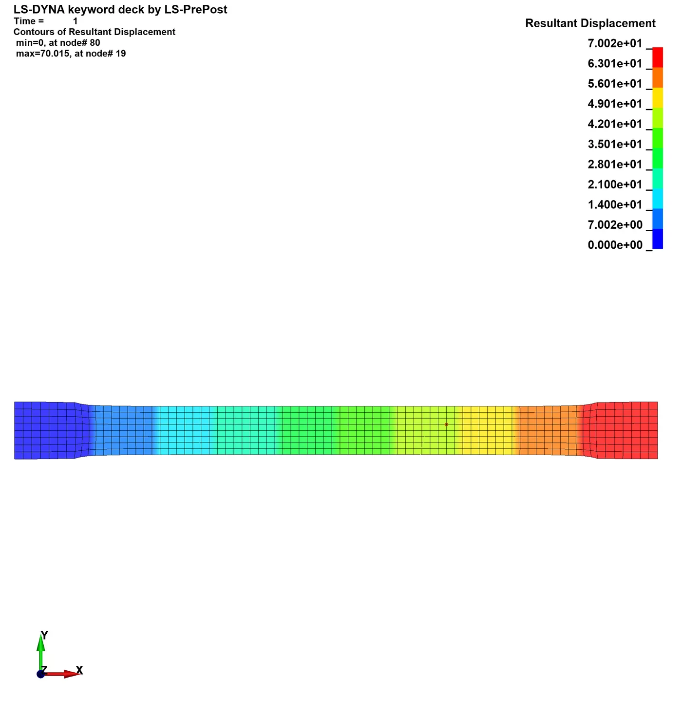
Analysis Setup:

Material model:

To get realistic results for any analysis using FEA, a good material model for the material is necessary. A material model can have all sorts of data describing the behaviour of the material in different conditions: say different tensile test curves for different strain rates and much more. This helps getting realistic behaviour of the component with the material model in all sorts of situations.

Building a material model requires test data from various experiments conducted in real life to describe the material behaviour in detail. A complex analysis would benefit from a detailed material model, whereas a simpler simulation would not benefit much. The data collected from an experimental test is first cleaned to make sure any unnecessary data points are filtered out to get clear picture. Usually the same test is repeated a number of times to ensure repeatability of the results. This test data is then inserted in the suitable format into a model: say effective stress-strain curve in x-y co-ordinates. A cleaner data with consistence behaviour in the case of a stress strain plot, inconsistent data points should be avoided as it can affect the stability if the simulation having such an material model. A fitted curve with 98%+ accuracy can solve such issues. After matching for the unit system of the analysis, this data can be added to the simple material model to make it more detailed – for example with the use of material model such as MAT24 – linear piecewise material.

A good practice of the material modelling procedure is the validation of the model. By performing simple analysis for which an experimental test can be performed or such data can be acquired, and then comparing the experimental and analysis results gives a good benchmark for the model. In this exercise, we try and replicate such a process.

Process:

1. Using the image provided for the true stress-strain curve for the graphite iron with the help of data digitizer tool. By first defining ‘x_0’, ‘x_max’ and ‘y_0’, ‘y_max’ and then selecting the points along the plot to get the x-y co-ordinates and hence the data-points.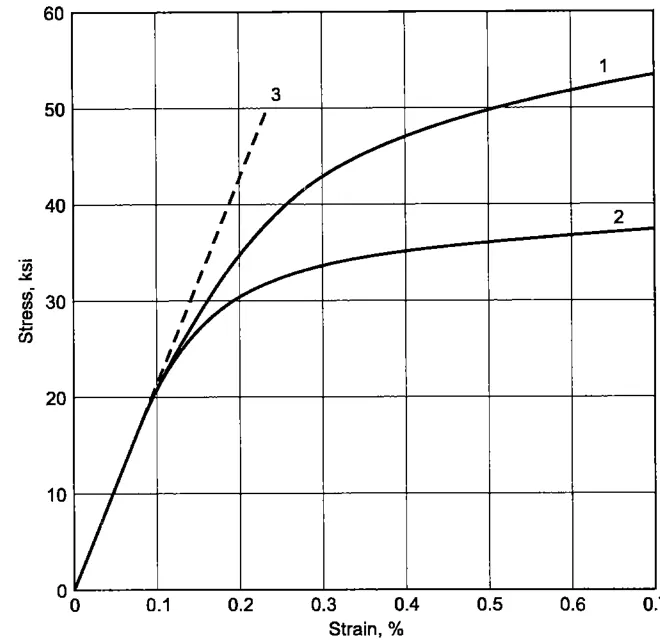

2. The true stress-strain data is then converted into effective plastic strain and stress to add to the material card. To keep the plot consistence, a curve is fitted to the extracted data, and the data-points are taken from the curve. Using the following relation the true stress-strain data is converted into effective plastic stress-strain data:

Effective stress = true stress

Effective strain = Total true strain - elastic true strain

= Total true strain - (true stress/Young's modulus)

for metals, 'E' is large(100x GPa), hence (true stress/E) can be taken as constant for all the points in the test data. This DOESN'T hold true for plastics where E is comparatively low (1x GPa).

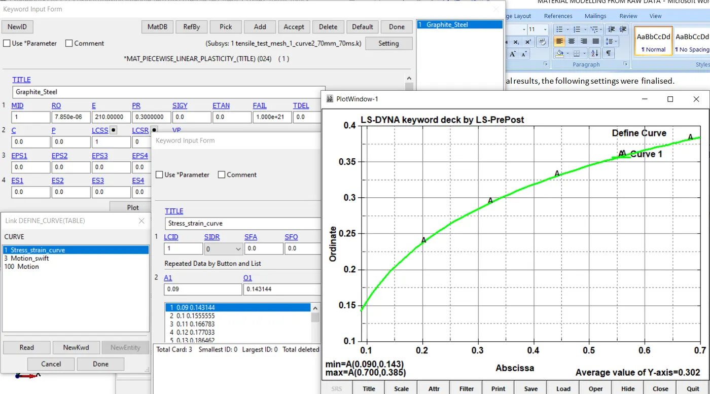
3. The acquired data is input as a curve, and then recalled in the material model- MAT24.

4. A tensile test model is setup for the given dog-bone model, where the boundary conditions are:

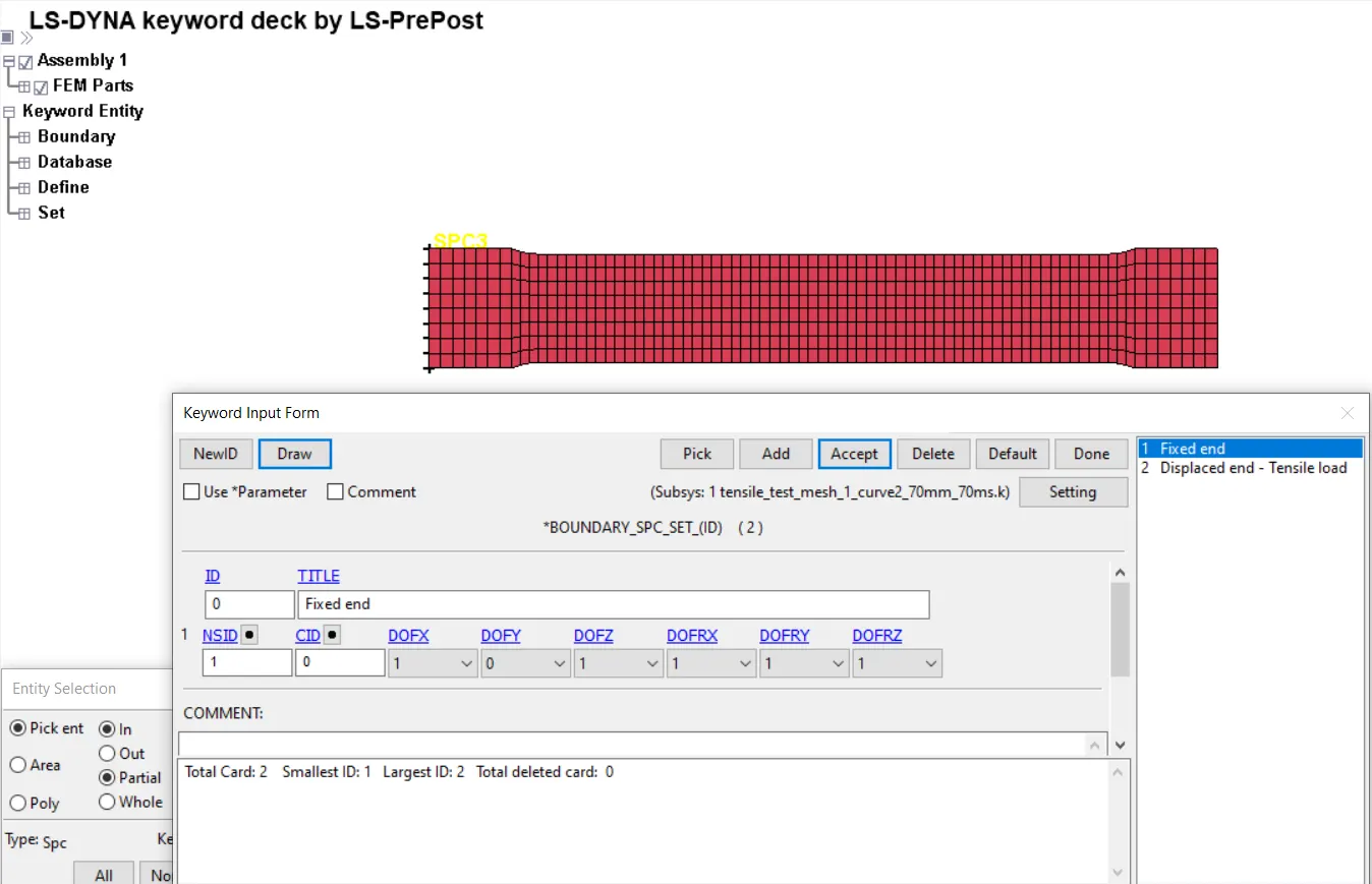
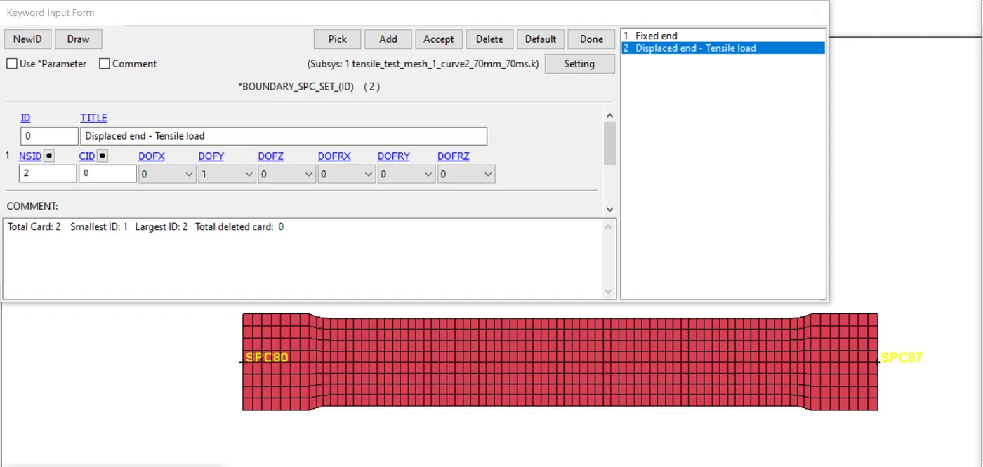
1. One end is fixed with all DOFs locked except translation in lateral direction to allow the compression.
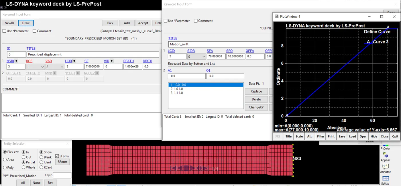
2. All nodes on the other end are added to a node_set to which a ‘prescribed_boundary_condition’ of displacement is applied in the longitudinal axis.
3. The middle node on each of the ends is constrained in all other DOF except translation in the longitudinal axis to avoid contradicting boundary conditions and keep the loading tensile in nature.

5. A linear displacement curve is defined to get cover good part of the experimental test with as much plastic straining as possible without getting into instabilities.

6. The necessary outputs were requested in ‘database’ keyword and the results were compared to the input curves.

7. To understand the process better an implicit analysis is performed for the same to observe the stress distribution, and overall results.

Procedure:

1. Acquiring the required data form experimental results:

Using the data digitizer the following data-points were collected from the given ‘True stress-strain plot’ for graphite iron specimen tensile test.

Curve_1 (true stress-strain)		Curve_2(True stress-strain)
strain(percentage)	stress(KSI)	strain(percentage)	stress(KSI)
0.006776601	1.075269	0.01307575	2.365591398
0.008073878	1.935484	0.019381587	3.76344086
0.014346279	2.795699	0.026951265	5.483870968
0.018131119	3.655914	0.037028567	7.52688172
0.023159739	4.516129	0.044604932	9.35483871
0.025700797	5.376344	0.054682234	11.39784946
0.028235168	6.129032	0.063515755	13.44086022
0.032006633	6.774194	0.07360643	15.69892473
0.035791473	7.634409	0.086171294	17.74193548
0.042083935	8.817204	0.088745787	19.13978495
0.04964024	10.32258	0.100040122	20.75268817
0.054675547	11.29032	0.113855454	22.90322581
0.062245225	13.01075	0.12265554	24.40860215
0.067307281	14.4086	0.136464184	26.4516129
0.077364521	16.12903	0.149022361	28.38709677
0.083690419	17.84946	0.169056599	30.53763441
0.09626197	20	0.179120526	32.3655914
0.107583052	22.04301	0.19540336	34.19354839
0.126380196	24.30108	0.212929974	36.02150538
0.142656342	26.02151	0.229199433	37.6344086
0.153930616	27.31183	0.250464077	39.56989247
0.173924731	28.8172	0.27420291	41.29032258
0.190160755	29.89247	0.289195153	42.3655914
0.208884342	30.96774	0.30791874	43.44086022
0.232569678	31.82796	0.327872733	44.30107527
0.256248328	32.58065	0.341601134	45.05376344
0.27493848	33.11828	0.361548441	45.80645161
0.294872412	33.65591	0.381502434	46.66666667
0.322262344	34.08602	0.403930616	47.31182796
0.348415182	34.62366	0.423871235	47.95698925
0.380786926	35.16129	0.443825229	48.8172043
0.408170171	35.48387	0.468734286	49.35483871
0.43305248	35.5914	0.498631841	50.10752688
0.460429038	35.80645	0.52229043	50.53763441
0.482830471	36.02151	0.547199486	51.07526882
0.510213716	36.34409	0.569614294	51.50537634
0.536339806	36.45161	0.594516664	51.93548387
0.558747927	36.77419	0.614443909	52.3655914
0.588612047	36.98925	0.633114	52.58064516
0.612257262	37.2043	0.656779276	53.11827957
0.637139571	37.31183	0.68291874	53.44086022
0.660778099	37.41935	0.699101268	53.65591398
0.694380249	37.74194

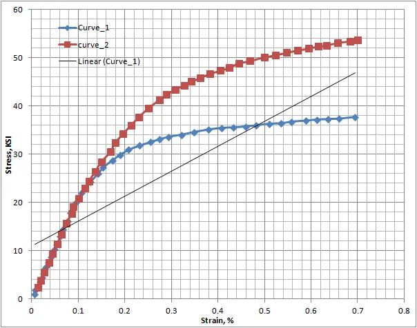
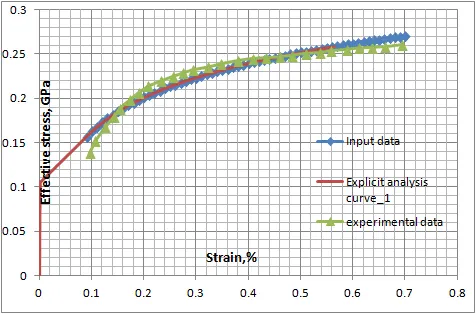
From the plot it can be observed that there are some inconsistencies in the plot hence a curve is fitted to it using trend-line feature in excel. It is made sure that the error is minimal. Given the nature of the graph, a logarithmic distribution gets a very close fit and hence is selected.

To match a suitable unit system, the units for stress were converted from KSI – Kilo pounds per square inch into GPa – Giga Pascal using following conversions:
1 Kilo Pounds per square inch = 4.44822 KN = 6.8947572 Pascal.

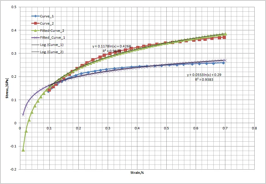
The finalised data comes out as:

	Curve_1		Curve_2
Effective strain	Effective stress[Gpa]		Effective stress[Gpa]
0.01	0.0353341	-0.11569
0.02	0.0736651	-0.03404
0.03	0.0960873	0.013727
0.04	0.1119962	0.047616
0.05	0.124336	0.073903
0.06	0.1344184	0.09538
0.07	0.1429429	0.113539
0.08	0.1503272	0.129269
0.09	0.1568406	0.143144
0.1	0.162667	0.155555
0.11	0.1679377	0.166783
0.12	0.1727494	0.177033
0.13	0.1771758	0.186462
0.14	0.181274	0.195192
0.15	0.1850893	0.203319
0.16	0.1886582	0.210922
0.17	0.1920108	0.218063
0.18	0.1951716	0.224797
0.19	0.1981616	0.231166
0.2	0.2009981	0.237208
0.21	0.2036962	0.242956
0.22	0.2062687	0.248436
0.23	0.2087269	0.253672
0.24	0.2110805	0.258686
0.25	0.2133379	0.263495
0.26	0.2155068	0.268115
0.27	0.2175939	0.272561
0.28	0.219605	0.276845
0.29	0.2215455	0.280978
0.3	0.2234203	0.284972
0.31	0.2252336	0.288835
0.32	0.2269893	0.292575
0.33	0.228691	0.2962
0.34	0.2303418	0.299716
0.35	0.2319448	0.303131
0.36	0.2335027	0.306449
0.37	0.2350178	0.309677
0.38	0.2364926	0.312819
0.39	0.237929	0.315879
0.4	0.2393291	0.318861
0.41	0.2406946	0.32177
0.42	0.2420272	0.324608
0.43	0.2433285	0.32738
0.44	0.2445998	0.330088
0.45	0.2458425	0.332736
0.46	0.247058	0.335325
0.47	0.2482473	0.337858
0.48	0.2494115	0.340338
0.49	0.2505518	0.342767
0.5	0.251669	0.345147
0.51	0.252764	0.34748
0.52	0.2538379	0.349767
0.53	0.2548912	0.352011
0.54	0.2559249	0.354213
0.55	0.2569396	0.356375
0.56	0.257936	0.358497
0.57	0.2589148	0.360582
0.58	0.2598766	0.362631
0.59	0.2608219	0.364645
0.6	0.2617513	0.366625
0.61	0.2626654	0.368572
0.62	0.2635646	0.370487
0.63	0.2644494	0.372372
0.64	0.2653203	0.374227
0.65	0.2661777	0.376054
0.66	0.267022	0.377852
0.67	0.2678536	0.379624
0.68	0.2686729	0.381369
0.69	0.2694802	0.383089
0.70	0.2702759	0.384784

2. Analysis Model and setup:

The given dog-bone specimen keyword file only has the mesh data and hence everything else needs to be added. To keep the analysis simple yet informative, the before mentioned boundary conditions were added along with a MAT24 material model consisting of the ‘log-data’ acquired from the experimental results. After trying a number of times to get the required results without any instability and unusual results, the following settings were finalised.

1. Explicit analysis:

1. PART, SECTION, MAT definition:

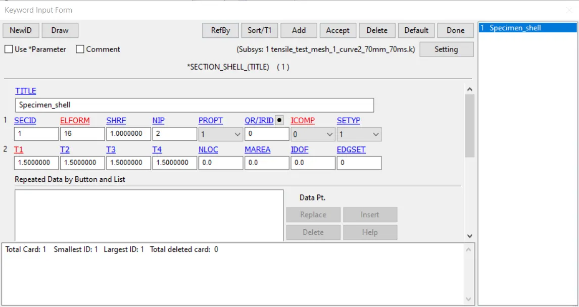
To get a comparative result, the section thickness of the specimen was kept 1.5mm in all the cases with an ‘elform’ of 16 - ‘Fully integrated shell element’ to get most details with more integration points along the thickness.

As mentioned, graphite steel material properties were used for the MAT24 linear piecewise plastic material card. The effective stress strain plot was defined using ‘define->curve’.

The input parameters were different for representation of the 2 curves describing different material structures.

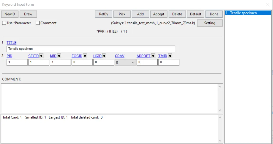
This is enough for the description of the specimen.

2. Boundary conditions:

As mentioned above the only boundary conditions defined were the SPCs to make sure the loading is purely tensile, and the prescribed displacement defined with a curve.

1. Fixed end with all DOF constrained except lateral translation:
2. Middle node on each end – free in longitudinal translation, constrained in all other DOFs.
3. Prescribed motion - displacement on the other end for tensile loading:

A liner curve is defined and called upon to impose the boundary condition using a set of nodes the other end from the fixed end.

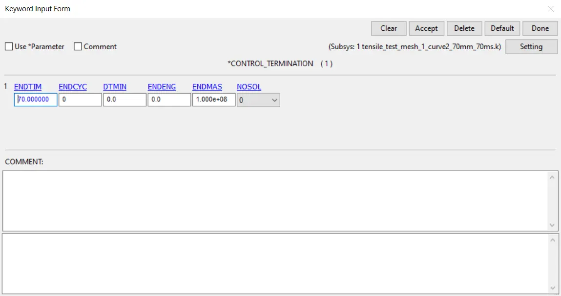
3. Database, control settings:

After trying a few short timed simulation runs giving out unrealistic outputs, for the sake of comparison a longer end time analysis is performed which yields more comparable results.

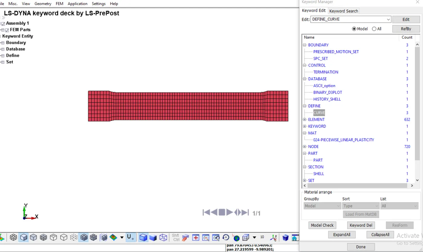
The usual output parameters were requested to get results which can be later compared.

Implicit Analysis:

To keep it simple, the run time was to be kept short and was finalised after trying out different iterations. As the implicit analysis requires implicit control cards to be enabled, the default parameters were used for fairness of the results. Only the initial time-step ‘dt0’ and the minimum ‘dtmin’ and maximum ‘dtmax’ time-step parameters were moved around.

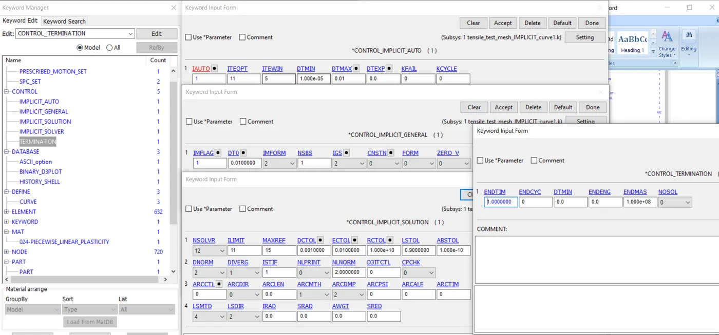
All the other parameters along with the material models were kept the same as the ones in explicit analysis.

Results:

Curve 1: Explicit analysis:

1ms analysis - short end-time analysis:

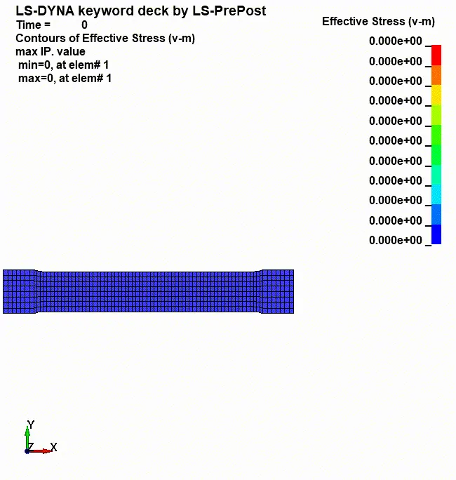
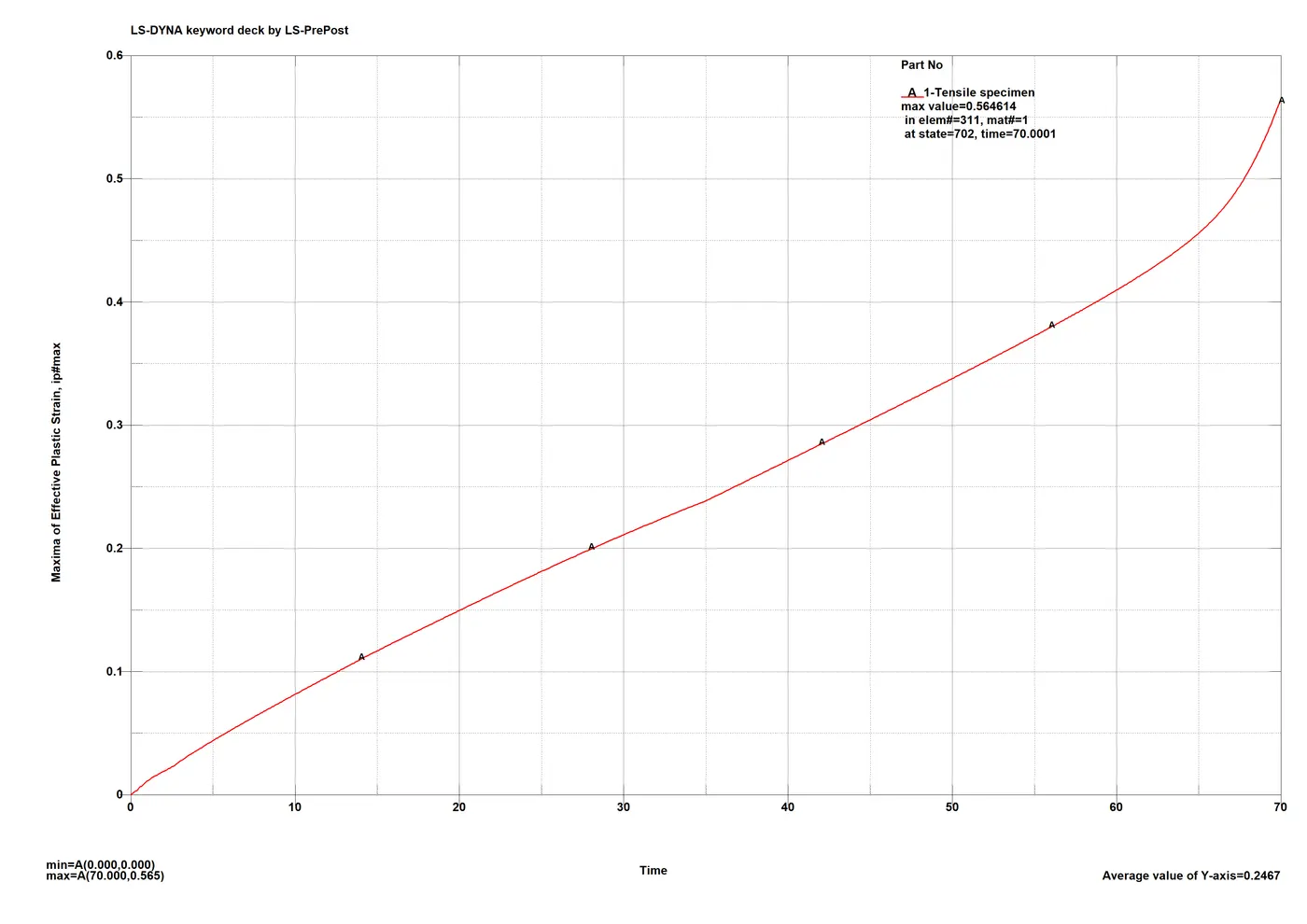
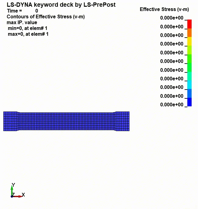
As mentioned before, due to the nature of explicit solver, the results acquired using a shorter end time (as used in implicit analysis) were very different and unrealistic – the stresses were being generated at the displacing end rather than the strained area. After making the end-time longer, better results were observed. A reason for that being tensile test is a static or quasi-static process, whereas explicit analysis and solvers are suitable for dynamic events.

70ms analysis - Long end-time analysis:

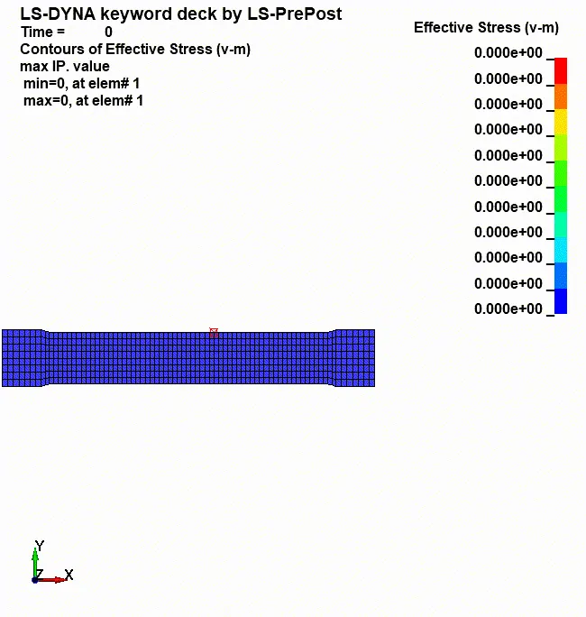
The propagation of stress wave can be seen in the result which is observed clearly in the shorter end-time case. The displacement B.C. is considered a ‘dynamic action’ by the explicit solver similar to a crash or impact test whereas in practice it is a quasi-static process, and hence the results are different and not considerable.

Things settle down a bit after the same analysis is run with a much longer end-time, and a linear loading – application of displacement B.C. As mentioned, the stress wave can still be seen propagating, reflecting through the specimen which again suggests explicit solver may not be the right option.

Effective stress:

Effective strain:

Effective stress v/s effective strain:

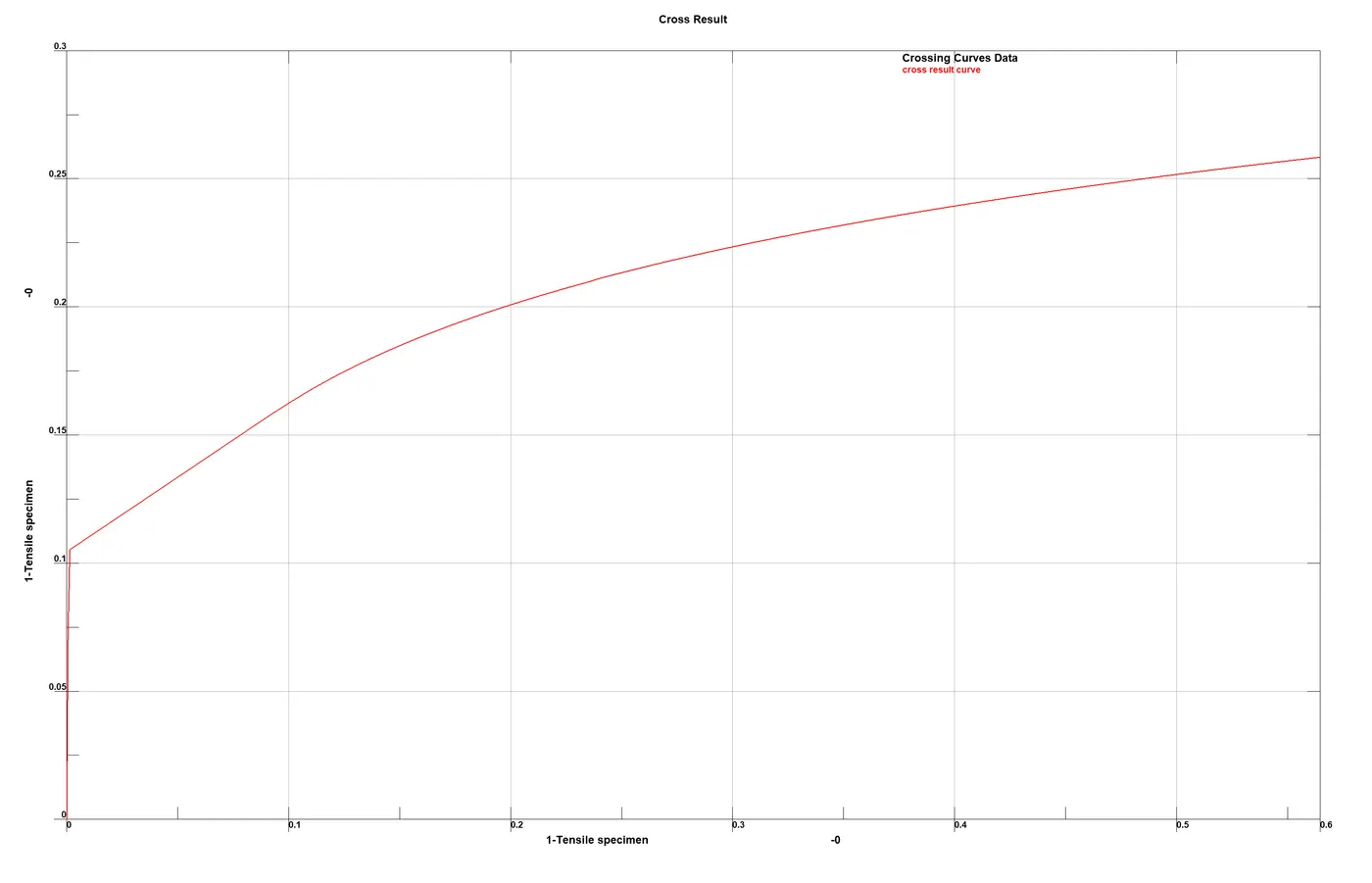
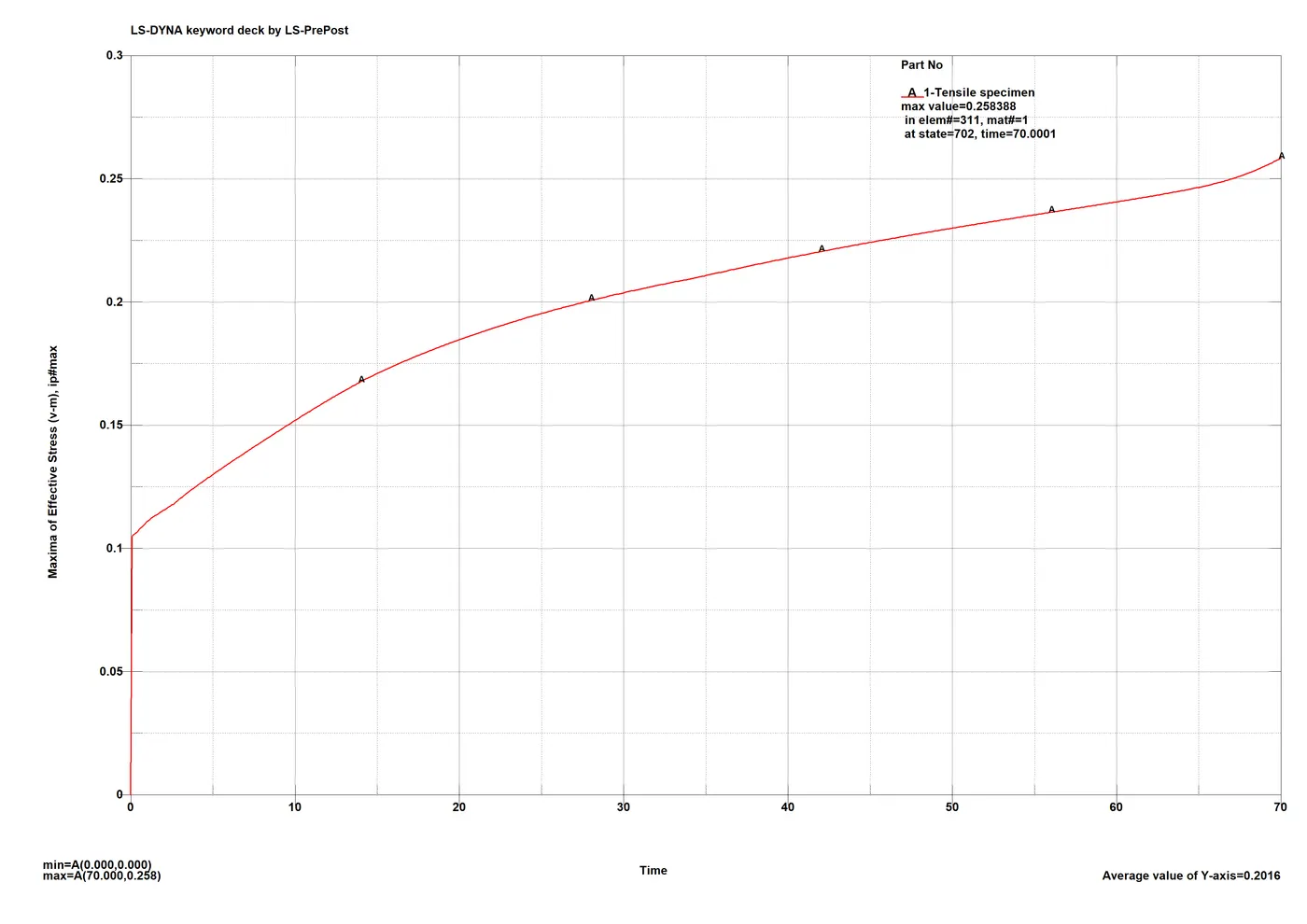
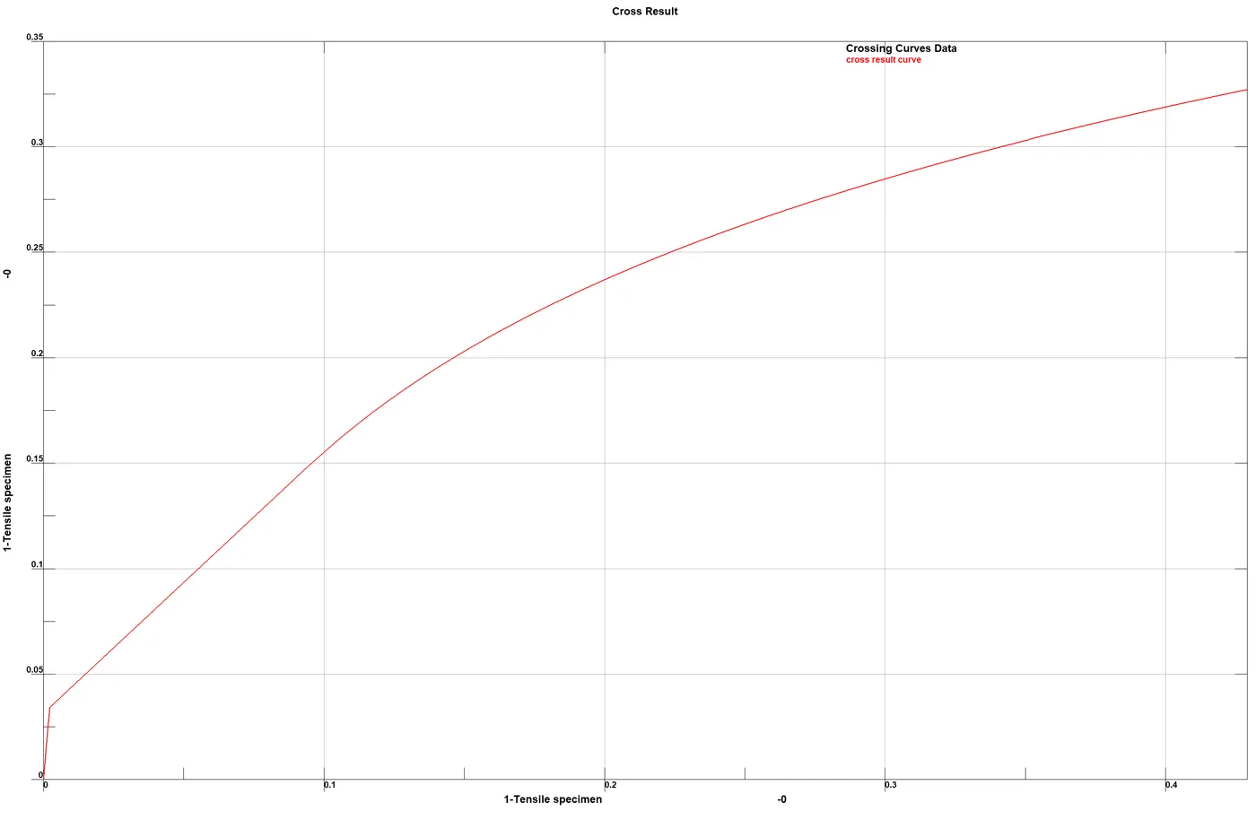
As expected the results closely mimic the input curves as the loading is linear in nature. Except the slight variation in the last 10ms of the analysis, the plots closely resemble the experimental data.

Curve 1: Implicit analysis:

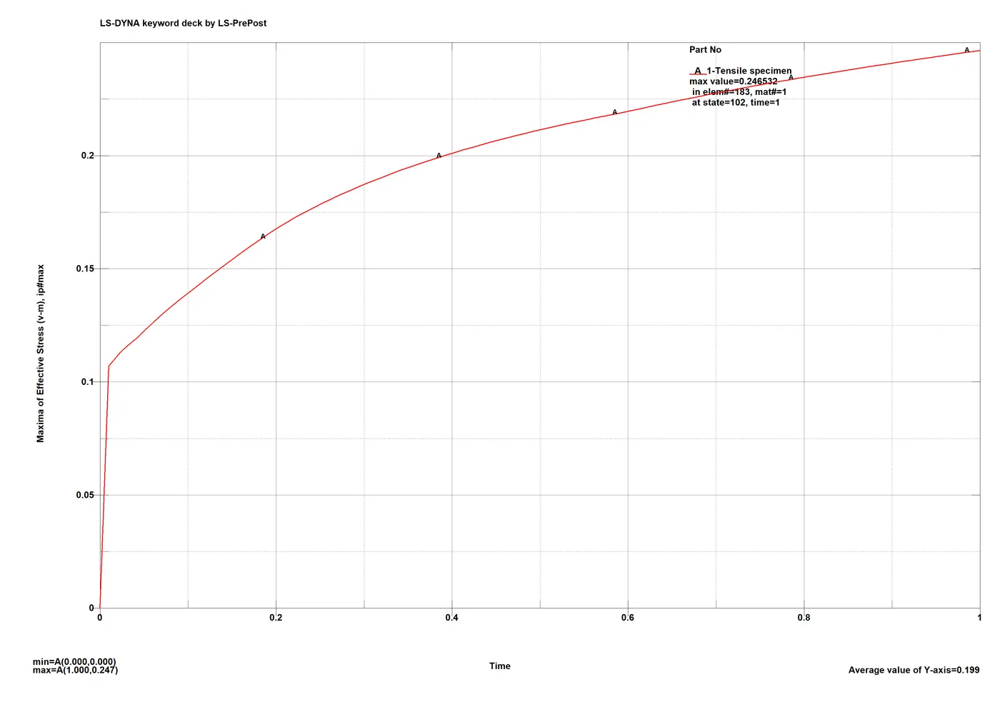
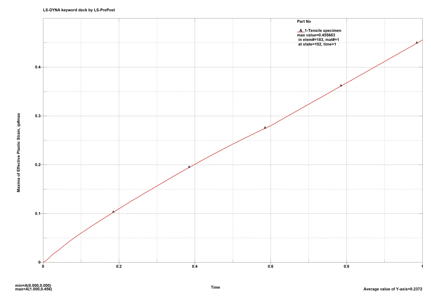
As mentioned, the run time for the analysis is kept low as implicit analysis tends to get into instabilities with non-linear simulations. Since the nature of the test itself is quasi-static, the results can be observed to have better progression. No visible stress wave propagation and stress concentration at the strained areas is observed, which was not well done during the explicit run.

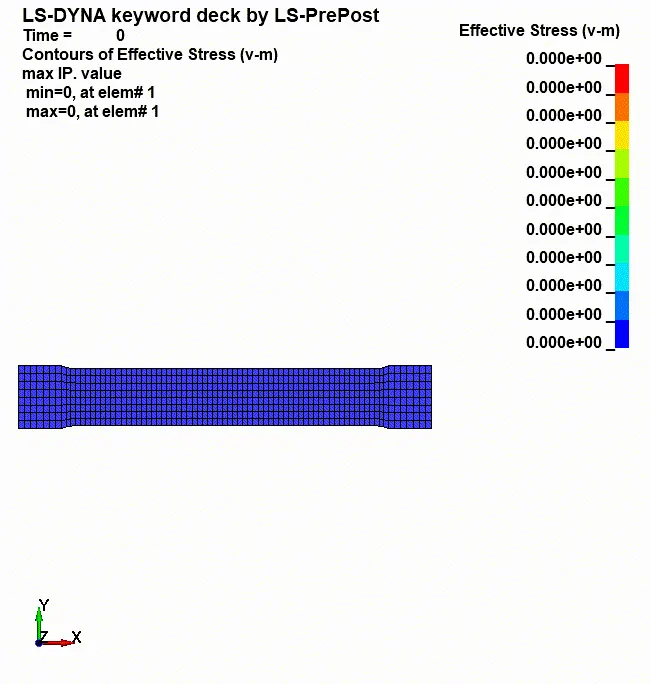
Effective stress:

Effective strain:

Stress-strain curve:

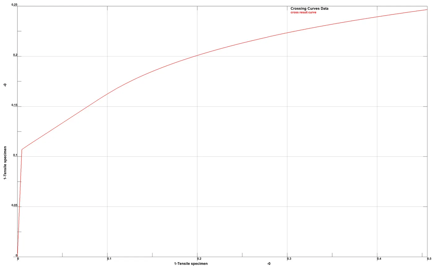
Similar to the explicit case, there is close resemplance to the input data, however the incostistancy at the end is there, giving it even better accuracy.

Implicit v/s explicit:

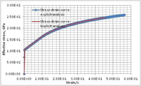
Hardly any difference can be observed between the two methods, but in hindsight the implic analysis gives better details as seen from individual curves.

Curve 2: Explicit analysis:

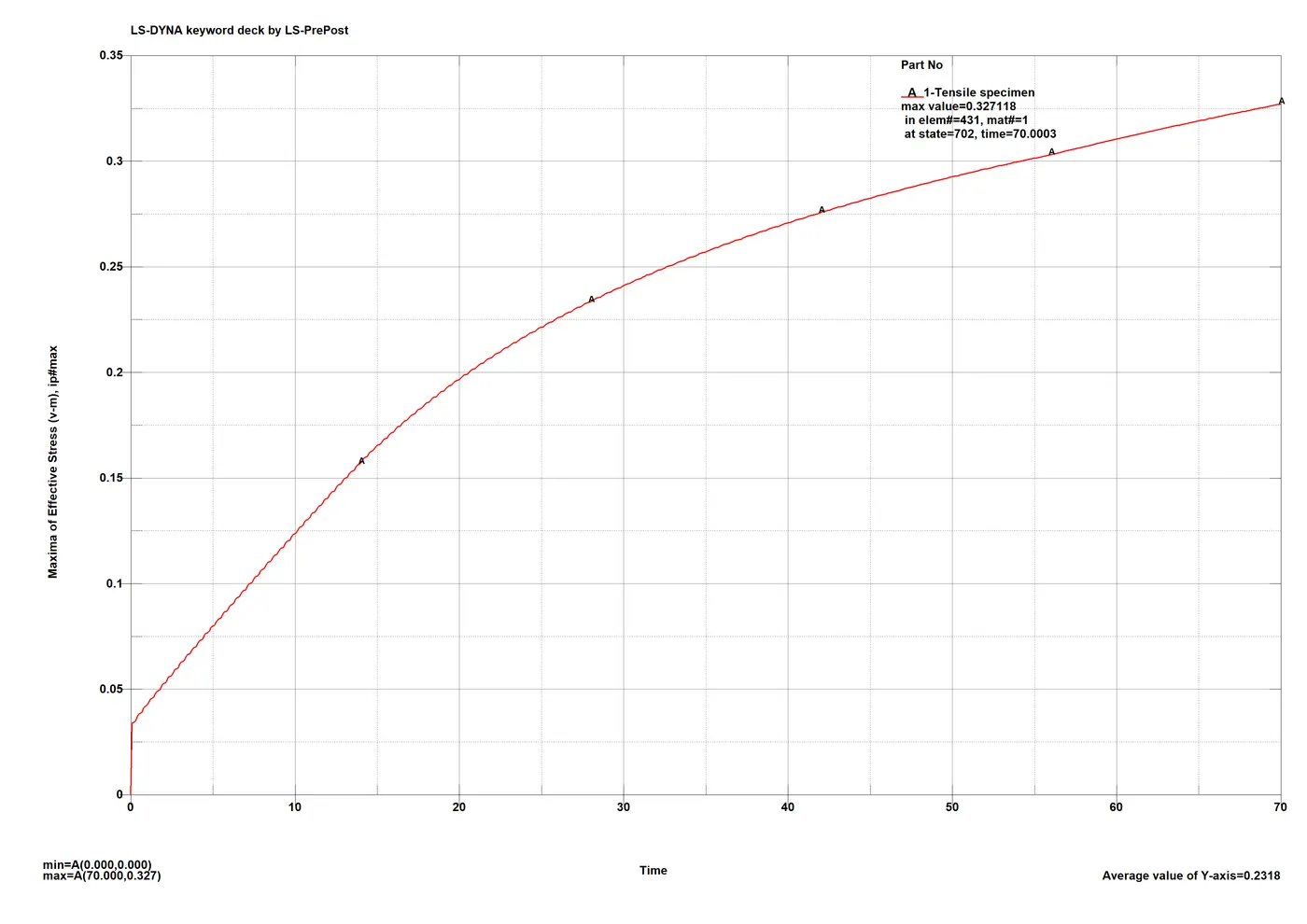
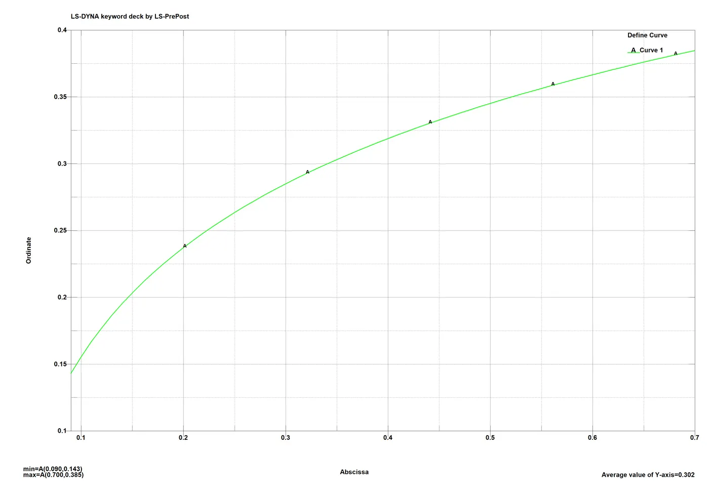
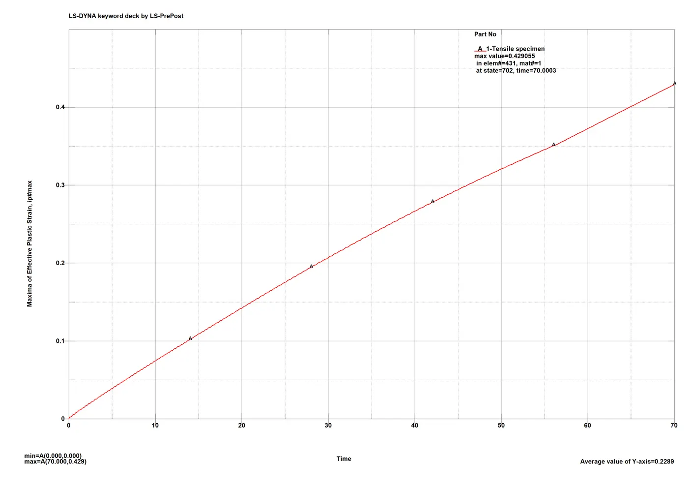
Similar results were observed as curve 1 for a short time analysis for the reasons mentioned before. The longer end-time analysis had similar story, with the stress wave propagation causing the stress concentration. The 2^nd curve has similar behaviour to the 1^st the difference being the stress figures. Possibly due to strain hardening the 2^nd curve showed higher stresses for the same percentage plastic strains. It was replicated in the results, as for essentially the same loading pattern, a greater resistance and hence stress is observed.

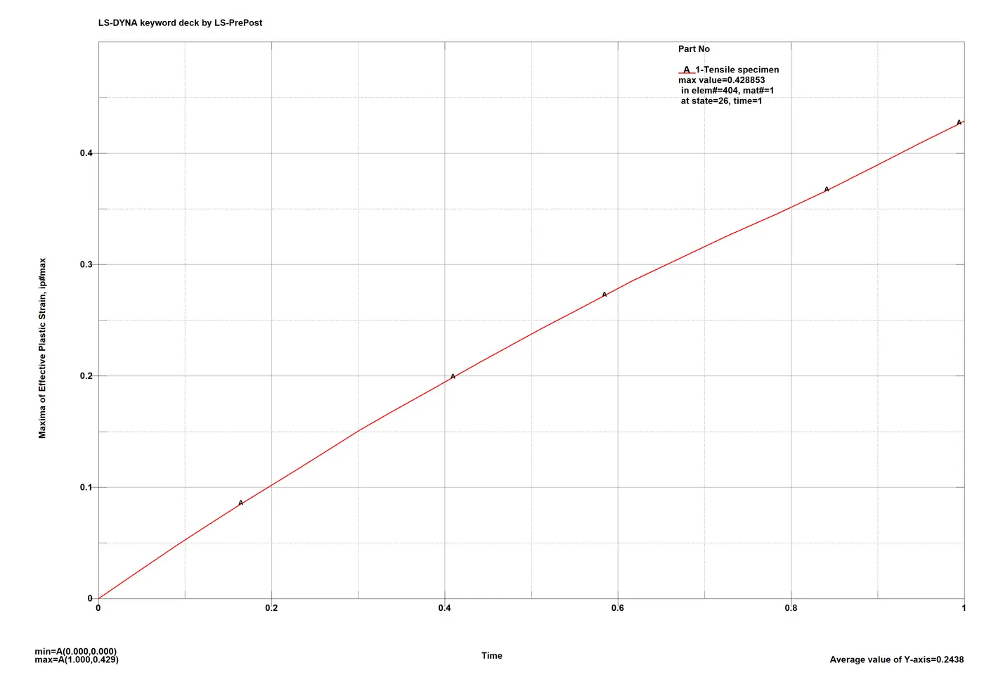
Effective stress:

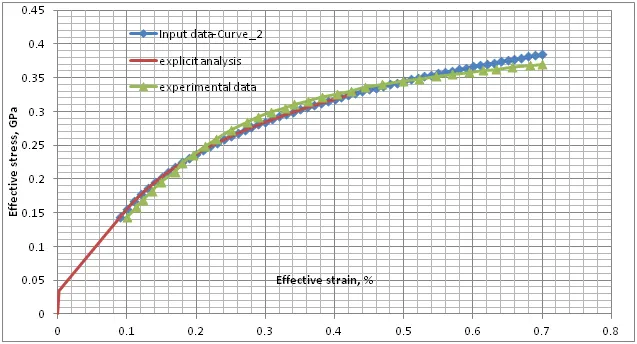
The output data resembles the input curve and the logarithmic behaviour as a result of linear loading.

i/p curve:

Effective strain:

Effective stress v/s effective strain:

As expected, there is a close resemblance between the input data and results from the analysis. The deviations are very small.

Curve 2: Implicit analysis:

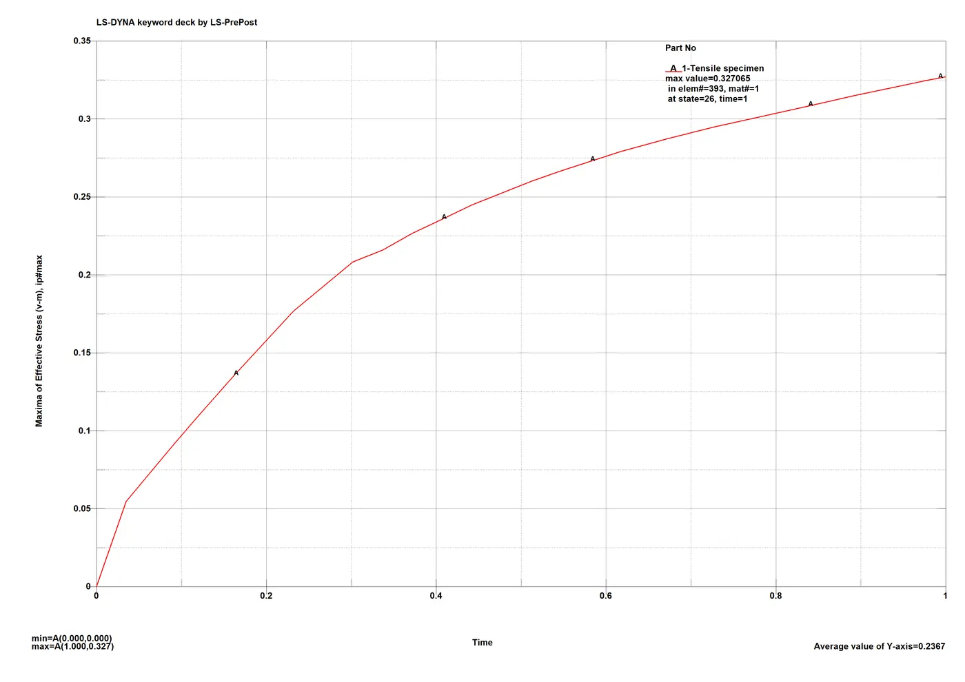
Due to numerical instabilities and high non-linearity of the analysis, the curve 2 analysis is a bit compromised. Less resolution in the output data leads to rough plots and uncertainty however, the behaviour of the plots makes resemblance clear. The contours for stress show logical results similar to curve – 1 again underline the superiority of implicit solvers for such simulations.

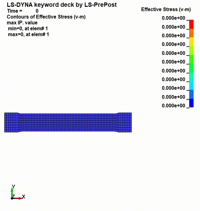
Effective stress:

Effective strain:

Effective stress v/s effective strain:

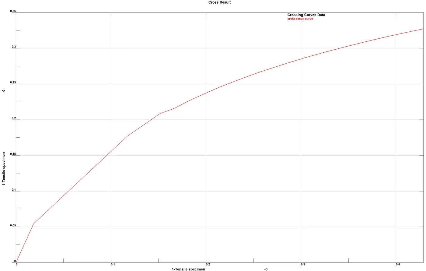
Lower resolution gives out a rougher plot, but the overall behaviour has resemblance with the input plot. The logarithmic nature of the plot makes the initial climb steeper as the fitted curve needs to match the majority of points in the middle region.

i/p curve:

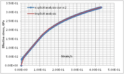
Implicit v/s explicit:

Only a slight deviation in the initial climb is the only noticable difference.

Conclusion:

1. Material modelling is one of the most important and influential part in CAE and its accuracy is essential for trustworthy results, hence the process should be done carefully with numerous validation simulations following it.
2. As this was just an study exercise, use of data digitizer is excusable. In practice, actual experimental data is essential. Data cleanup being one of the most important stage in the process, it is benifitial to have a large number of data points to start with, which was not possible in this case.
3. From the results and comparison, it is clear tha despite the small instability issues, implicit analysis or rather the solver is better suited for tests which are static or quasi-static in nature such as the tensile test. An explicit analysis will give comparable results but its purpose by design is to solve dynamic problems and hence is not reliable in such cases.
4. From the results it can be concluded that the material model build is fairly accurate and acceptable, however more validation tests are recommended.