week-11 Joint creation and Demonstration

Aim: To understand and demonstrate how different types of joints can be simulated using rigid and deformable bodies in LS Dyna.

Simulation setup:

There are various types of joints which can be simulated in LS Dyna for demonstration purposes as well as FEA analysis where stresses are induced due to motion. Most common types of joints include revolute joint, spherical joint, translational joint, cylindrical joint, planar joint etc. which can be defined between two or more rigid bodies in case of demonstrations or deformable bodies for FEA using ‘extra nodes’ method or ‘CNRB or constrained nodal rigid bodies’ method. For the extra nodes method, additional nodes are created to define the motion such as axis of rotation in case of a revolute joint, and then these nodes are added to the bodies to complete the joint. Then a ‘constrained joint’ is created where these nodes are called in and the joint is defined. There is a particular order which is taken care of in the calling of the nodes with respect to which body they belong to.

Common types of joints:

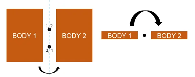
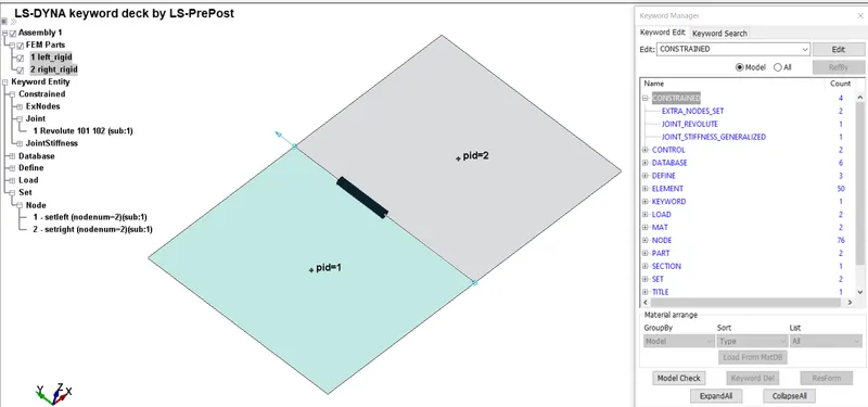
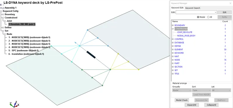
1. Revolute Joint: Defined to portray a joint between two bodies which permits only rotational motion about the joint axis. A good example would be hinged joint on doors and lids of containers. A set of nodes is required to define the axis about which the motion is to be simulated. The sequence of nodes can be seen in the picture below. The rotational motion is only allowed along the axis formed by two pair of coinciding nodes.

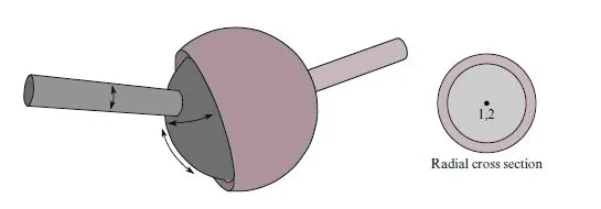
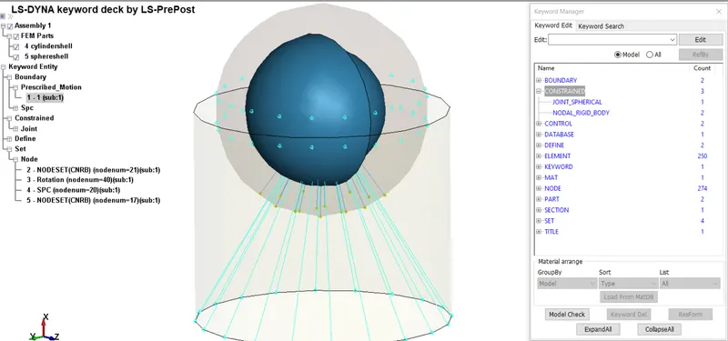
2. Spherical Joint: A ball and socket joint which allows the rotational motion of one body with respect to the other which can be seen in constant velocity joints, and ball joints. A single node is used in this case for each body to define the joint.

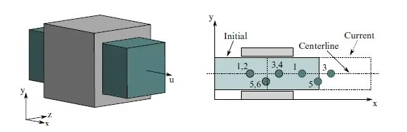
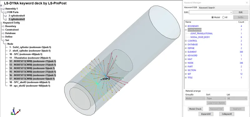
3. Translation Joint: Used to simulate translation motion along an axis in a single plane. Example for the joint type are piston-cylinder, slider-rail motion etc. A set of nodes are defined to fix the axis and the plane for the motion.

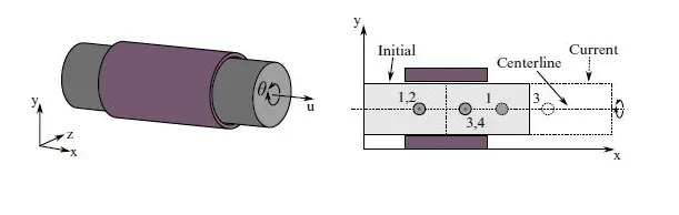
4. Cylindrical joint: A combination of spherical joint and translation joint, seen in screw and nut-bolt motion. A set of nodes is defined to fix the axis of rotation and the axis along which the translation is allowed.

Process:

The procedure for defining the joints is more or less the same for both rigid body joints and deformable body joints. As per the joint in question, a set of ‘extra’ nodes are to be created using which the axis or the point necessary for the joint is defined. Then these ‘extra’ nodes are made a part of the participating bodies such that the joint defined using these nodes can be extrapolated/associated to the respective bodies. As shown in the pictures above, a particular sequence is followed in selecting the nodes to define the joint in order to properly simulate the joint.

Procedure:

1. Rigid body joints:

a) The above mentioned process is followed as is for creation of a joint. In rigid body joints, the bodies as the name suggests are rigid bodies which are infinitely stiff. As a result no stresses and strains are generated due to the motion and the method is used mostly for motion simulation and not the FEA analysis. The required bodies are created using shape meshing option and are given the properties of rigid body by assigning MAT-20- rigid body material card to them.

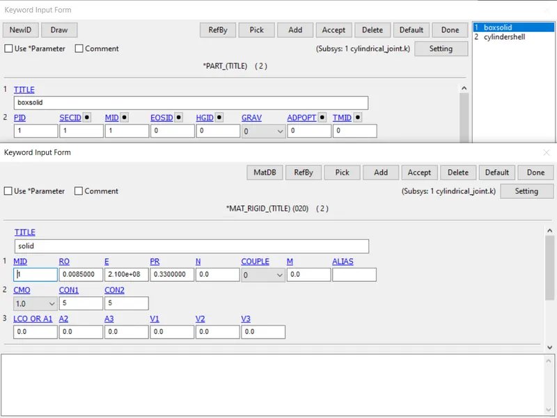
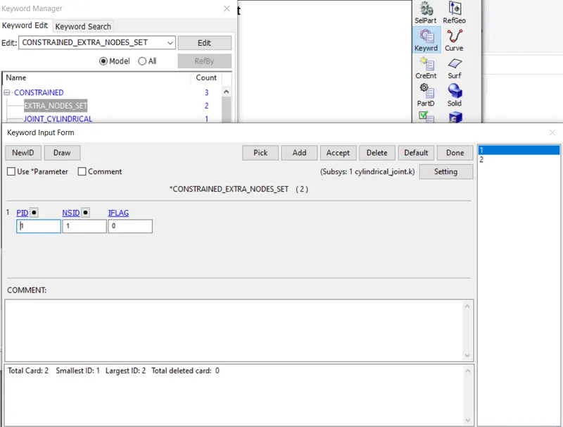
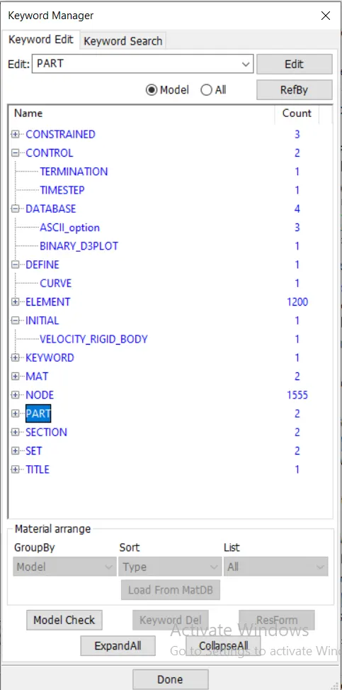
b) After defining the rest of the necessary parameters for the bodies, the respective joint is defied. As mentioned before, a set of ‘extra’ nodes are used to fix the necessary axis or plane for the required joint. The sequence of the selection of nodes is crucial as well as associating these node-sets with the respective bodies using ‘Extra_node_sets’ option.

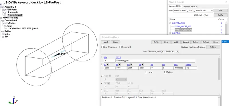
c) The joint is defined using ‘x_joint’ option. The nodes represent the axis about which the motion is allowed.

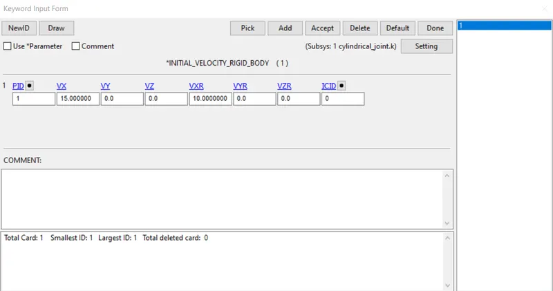
d) To simulate the motion a prescribed or initial boundary condition is applied which the joint has allowed, foe instant in this example an initial rotational velocity about y-axis and a translation motion along x-axis is defined to simulate the joint.

e) Finally the required outputs are requested along with defining the simulation setup keywords to fix the time step and end time settings.

2. CNRB joints: Constrained Nodal Rigid Body:

a) Similar to rigid body joints, these joints are defined using nodes using ‘x_joint’ option, same as the rigid body joints. The difference being the use of CNRBs to associate the nodes with the bodies. This essentially joins the nodes with the respective bodies rigidly and as a result there is no compulsion of assigning a rigid material to the bodies.

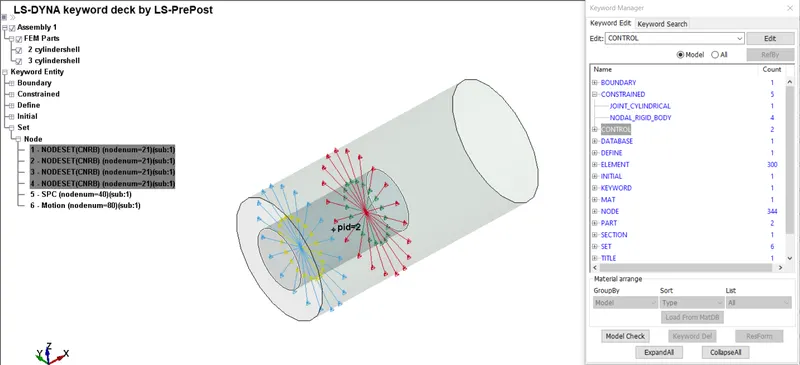
After defining the bodies rigidly joint to the nodes, these nodes are added to the joint card as mentioned and the required boundary conditions are also applied. Except the CNRB definition, and the body properties, the process used for both the types of joints is identical.

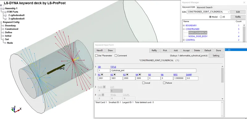
Following are the various joints using both the rigid body and CNRB methods and their simulations:

1. Revolute Joint:

a) Rigid body method:

b) CNRBs method:

2. Translation Joint:

a) Rigid body method:

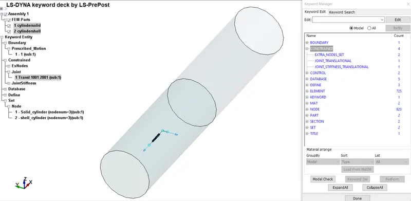
b) CNRBs method:

3. Spherical Joint:

a) Rigid body method:

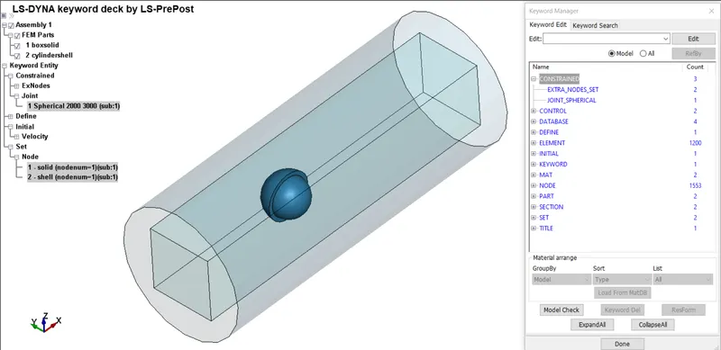
b) CNRBs method:

4. Cylindrical Joint:

a) Rigid body method:

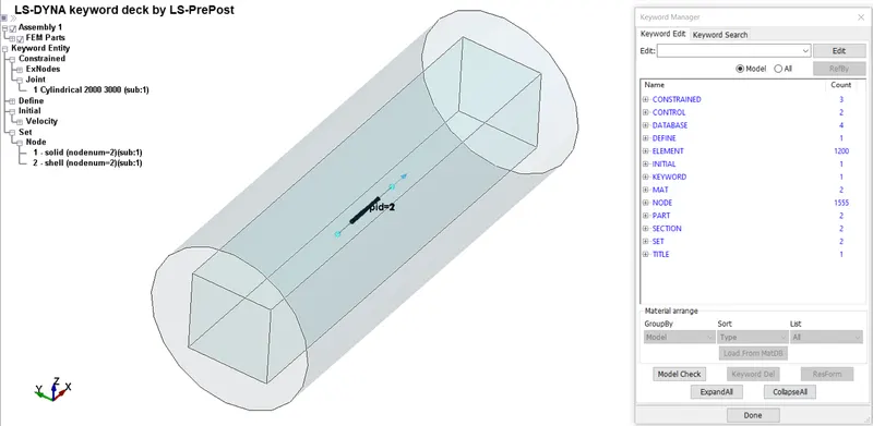
b) CNRBs method:

Conclusion:

Using extra nodes method we can simulate all the major types of joints for rigid as well as deformable bodies using the rigid body or the CNRB method.

Report Word file link:

https://drive.google.com/file/d/17Idd-wuNNkoLINlfzAsf1N2F8Dh0PACr/view?usp=sharing

**Due to an error the GIF files showing the simulation results are not getting uploaded, please find them in the attched files report.**