Understanding and implementing 2 DOF transient handling (Bicycle model) model for various examples and build a 4 wheel steer model based on the same

Introduction to 2DOF transient handling model:

The cornering behaviour of vehicle is termed as handling. 'Handling' implies the responsiveness of a vehicle to driver input or the ease of control. It is essentially a measure of a vehicle-driver combination meaning that the driver observes the vehicle direction and position and corrects his input to achieve the desired motion. For this purpose, an open-loop relation between vehicle response and steering inputs is used. The objective is to understand the directional response of the vehicle and how various design parameters influence this. A 2-DOF Model known as the Bicycle Model is representation of the automobile which takes into account only 2 degrees of freedom- Yaw and Lateral movement. Both steady-state and transient-state responses can be studied using this model. In transient system vehicle behaviour changes with time and hence is more practical approch to a handling model.

Assumptions:

• The height of vehicle CG is at ground level
• No longitudinal load transfer.
• No lateral load transfer (since no track width).
• Linear range tires.
• Constant forward velocity.
• No chassis or suspension compliance effect.

The basic equations for forces and moments acting on a rigid body due to acceleration of the body are:

F = m*a

T = I*α

Free body Diagram:

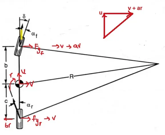
Here,

u - Longitudinal velocity of the vehicle

v - Lateral speed

r - Yaw rate

δ - Steering angle

αf , αr - front and rear slip angles.

Force balance equation:

Fyf + Fyr = m(v'+ur)

Moment balance equation:

Izz*r = fyf*a - fyr*b

and,

αf = δf - tan^-1((v+a*r)/u)

αr = δr- tan^-1((v+b*r)/u)

State space representation:

It is the linear representation of the dynamic system in either continuous or discrete form

or

It is a representation of mathematical model of a physical system as a set of input, output and state variables related by first-order differential equations.

x' = A*x + B*u

y' = C*x + D*u

where,

A - System matrix B - Input matrix

C- Output matrix D - Feed forward matrix

It can be expressed in the form of differential equations

`(dx_1)/dt=a_11 x_1+a_12 x_2+b_1 v(t)`

`(dx_2)/dt=a_21 x_1+a_22 x_2+b_2 v(t)`

`y=C_1 x_1+C_2 x_2+d_1 v(t)`

Converting these equations to matrix form:

`[[dotx_1], [dotx_2]]=[[a_11,a_12],[a_21,a_22]][[x_1], [x_2]]+[[b_1],[b_2]]cdotv(t)`

`y=[[C_1,C_2]][[x_1],[x_2]]+d_1 v(t)`

Writing governing equations in state space format:

`d/dt [[V],[r]]=[[-(C_(∝f)+C_(∝r))/(m*u),(bC_(∝r)-aC_(∝f))/(m*u)-u],[(bC_(∝r)-aC_(∝f))/(I_z u),(-(a^2 C_(∝f)+b^2 C_(∝r)))/(I_z u)]][[V],[r]]+[[C_(∝f)/m],[(aC_(∝f))/I_z]].[δf]`

There are three outputs for this model:

Yaw rate (r)

Lateral velocity (v)

Lateral acceleration (dv/dt)

[Yyawrate] = [0 1] `[[V],[r]]` + [0]δ

[Ylateral rate] = [1 0]`[[V],[r]]` + [0]δ

[Yacceleration] = `[[-(C_(∝f)+C_(∝r))/(m*u),(bC_(∝r)-aC_(∝f))/(m*u)-u]]` + u [0 1]

The only change in the code for Rear wheel and 4 wheel steer vehicles is the B matrix.

B= `[[C_(∝r)/m],[(aC_(∝r))/I_z]].[δr]` – Rear wheel steering

B= `[[C_(∝f)/m,(C_(∝r))/m],[(aC_(∝f))/I_z,(-bC_(∝r))/I_z]].[[δf],[δr]]` – All wheel steering

Derivative Notation of the Bicycle Model:

The derivatives are slopes of force/moment curves against motion variables β, r and δ. They relate forces and moments to small variations of the variables mentioned. In this model, they can be considered separately, but, as a group these variables define the unbalanced forces and moments arising out of the tyres.

The equations describing the derivative notation of the bicycle model are:

`m⋅u⋅((dβ)/dt) + m⋅u⋅r = (Cαf+Cαr)⋅β + (a⋅Cαf - b⋅Cαr/u)⋅r − Cαf⋅δ`

`Izz⋅((dr)/dt) = (a⋅Cαf−b⋅Cαr)⋅β + ((a^2⋅Cαf+b^2⋅Cαr)/u)⋅r - a⋅Cαf⋅δ`

Yawing Moment Derivatives:

a) Control Moment Derivative:

Nδ = a⋅Cαf

It is the proportionality factor between the yawing moment and the steering angle (δ). It increases with the cornering stiffness of the front tires (Cαf) and their distance from the C.G.(a). The control moment derivative is always positive.

b)Yaw Damping Derivative:

Nr = (a²⋅Cαf + b²⋅Cαr)/u

It is the proportionality factor between the yawing moment and the yawing velocity(r) of the vehicle. Yaw damping is always negative, hence the term damping in the linear range of tyres. It is exactly analogous to an angular viscous damper i.e. it tries to reduce the yawing velocity.

c) Static Directional Stability (Under Steer/Over Steer) Derivative:

Nβ = a⋅Cαf − b⋅Cαr

It is the difference between the moments about the C.G. produced by the front and rear wheels. With a positive Nβ, the vehicle is always trying to align itself, hence under-steer.

Lateral Force Derivatives:

a)Control Force Derivative:

Yδ = Cαf

It is the proportionality factor between side force due to steering and the steer angle and is always positive.

b) Damping in side slip derivative:

Yβ = Cαf + Cαr

It is similar to the slope of lateral force vs slip angle curve for the entire vehicle where there is a linear zone, translational zone and a sliding zone.

c) Lat force/yaw coupling derivative:

Yr = (a⋅Cαf − b⋅Cαr)/u

This is the side force due to yaw velocity. It arises from the difference in lateral tyre forces that comprise the yaw damping derivative

1.

1. Un-damped Natural frequency: w_n = [ y_B*N_R + N_B*M*u – y_R*N_B ]/ [M*u*I_zz]

here, y_B = Cf + Cr

N_R= (a^2*Cf + b^2*Cr)/u

N_B = (a*Cf - b*Cr)

y_R = (a*Cf - b*Cr)/u

Considering the case at 60 ft/sec

a) Passenger Car:

1) Un-Damped Natural frequency calculation:

y_B = 13752 + 11460 = 25212 lbs/rad,

N_R = (2.92^2*13752 + 5.41^2*11460)/60 = 7,544.45798 lbs-ft-sec/rad,

N_B = 2.92*13752 – 5.41*11460 = 21,842.76 lbs-ft/rad,

y_R = 21842.76/60 = 364.046 lbs-sec/rad

Taking mass M in slugs, M = 2000*0.453592/14.594 = 62.16 slugs, and I_zz in slug-ft^2

I_zz = (1128/14.594)*11.11 = 832 slug-ft^2

w_n^2 = [(-25212*-7544.458) + (21842.76*62.16*60) - (-364.046*21842.76)] / [62.16*60*832 ]

= 87.66 (rad/sec)^2

W_n = 9.36 rad/sec = 9.36/6.28 = 1.49044 Hz.

2) Damping Ratio:

ζ = C / C_critical = C / 2sqrt(k*I_zz ) = C / 2*I_zz*W_n

and C = -[N_R + (I_zz*y_B)/ M*u] = 13173 lbs-s/ft, C_critical = 2* I_zz*W_n =15575.04 lbs-s/ft

ζ = 15575.04/13173 = 0.8453

3) Damped frequency calculation:

W = W_n*sqrt(1- ζ^2) = 9.36*sqrt(1-0.8453^2) = 5.0054 rad/sec = 0.7970 Hz

Matlab code for 2 DOF bicycle model :

clear all;
%Transient 2 wheel handling simulation with 2 wheel steering for a Passanger Car

m = 2000; %total weight in lbs
mf = m*0.65; %Front weight bias in lbs
mr = m-mf; %rear weight bias in lbs
Iz = 8158.84; %Yaw moment of Inertia in slug-ft^2
l = 8.33; %wheelbase in ft
a = 2.92; %front axle to C.G.in ft
b = l-a; %rear axle to C.G. in ft
g = 315.6274163386; %ft/s^2

%Transient 2 wheel handling simulation with 2 wheel steering for an F1 Car
%m = 1719; %total weight in lbs
%mf = m*0.4; %Front weight bias in lbs
%mr = m-mf; %rear weight bias in lbs
%Iz = 6256.56; %Yaw moment of Inertia in slugs-ft^2
%l = 9.52; %wheelbase in ft
%a = 5.71; %front axle to C.G. in ft
%b = l-a; %rear axle to C.G. in ft
%g = 315.6274163386; %ft/s^2

%Cf = 62228; %Frontnt cornering stiffness in lbs/rad
%Cr = 96608; %Rear cornering stiffness in lbs/rad

Cf = 13752; %Fornt cornering stiffness in lbs/rad
Cr = 11460; %Rear cornering stiffness in lbs/rad
u = 60; % ft/sec
k = (mf/Cf)-(mr/Cr);

%Defining the state space equation matrices

A = [-(Cf+Cr)/(m*u), ((b*Cr-a*Cf)/(m*u))-u;
    (b*Cr-a*Cf)/(Iz*u), -(a^2*Cf + b^2*Cr)/(Iz*u)];
  

% Input Matrix
B = [Cf/m;  a*Cf/Iz];

% Output Matrix
C_lat = [1 0]; D_lat = 0; % Lateral velocity
C_yaw = [0 1]; D_yaw = 0; % Yaw rate
C_accl = A(1,:) + u*[0 1]; D_accl = B(1); %Lateral acceleration

C = [C_lat; C_yaw; C_accl];
D = [D_lat; D_yaw; D_accl];

t = [0:0.01:6];
I = (5*pi/180)*sin(7*2*pi*t); %Input steering angle of 5 deg at 7 Hz.

pkg load control;
 
sys = ss(A,B,C,D); %state space representation
S = lsim(sys,I,t); %Defining the sinusoidal input

sys.inputname = {'steering angle'};
sys.outputname = {'lateralV';'yawV';'acclat'};

yg = (u/l)/(1+((k*u^2)/(57.3*l*g))); % yaw gain

figure(1) 
[mag,w]= bodemag(sys({'yawV'},'steering angle')); %Frequency response calculation
s_in = (w/6.28);
s_in_tr = transpose(s_in);
yg_tr = [mag]./[s_in_tr];

loglog(s_in,[mag],'linewidth',3); grid on;
set(gca,'fontsize',18);
xlabel('Frequency in Hz');
ylabel('Yaw rate in deg/sec');

figure(2) %Step Response plot
step(sys);
hold on

figure(3) 
subplot(2,1,1)
grid on
plot(t,S(:,1),'g','linewidth',2); %Sine Response for lateral speed 
set(gca,'fontweight','bold')
title('Lateral Speed Sine Response- Passenger Car','fontsize',15)
xlabel('Time (sec)');
ylabel('Lateral speed (ft/sec)')
hold on


subplot(2,1,2) 
grid on
plot(t,S(:,2)*180/pi,'g','linewidth',2); %Sine Response for yaw rate
set(gca,'fontweight','bold')
title('Yaw Rate Sine Response- Passenger Car','fontsize',15)
xlabel('Time (sec)');
ylabel('Yaw Rate (deg/sec)')
hold on


figure(4)
subplot(2,1,1) 
grid on
plot(t,S(:,3),'g','linewidth',2); %Sine response for lateral acceleration
set(gca,'fontweight','bold')
title('Lateral Acceleration Sine Response- Passenger Car','fontsize',14)
xlabel('Time (sec)');
ylabel('Lateral Acceleration (ft/sec^2)')
hold on


subplot(2,1,2) 
grid on
plot(t,I*180/pi,'g','linewidth',2); %Sine response for steering
set(gca,'fontweight','bold')
title('Steering Angle- Passenger Car','fontsize',15)
xlabel('Time (sec)');
ylabel('Steering Angle(deg)') 


figure(5)
loglog(s_in,yg_tr,'linewidth',3); grid on;
set(gca,'fontsize',18);
xlabel('Frequency in Hz');
ylabel('Yaw gain in (deg/sec)/deg');

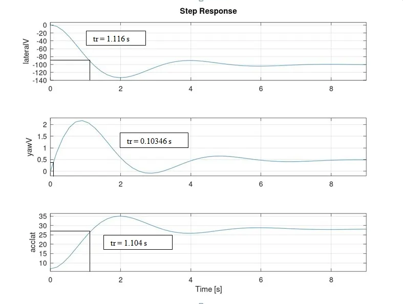
4) Rise time calculation from the step response plot:

b) F1 car:

1) Un-damped Natural frequency:

y_B = 62228 + 96608 = 158836 lbs/rad,

N_R = (5.71^2*62228 + 3.81^2*96608)/60 = 57,187.6553 lbs-ft-sec/rad,

N_B = 5.71*62228 – 3.81*96608 = 12754.6 lbs-ft/rad,

y_R = 12754.6 /60 = 212.576 lbs-sec/rad

Taking mass M in slugs, M = 1719*0.453592/14.594 = 53.38 slugs, and I_zz in slug-ft^2

I_zz = (865/14.594)*11.11 = 639 slug-ft^2

w_n^2 = [(158836*57,187.6553) + (12754.6*53.38 *60) - (212.576 *12754.6)] / [53.38 *60*639]

= 4417.1 (rad/sec)^2

W_n = 66.461 rad/sec = 66.461/6.28 = 10.583 Hz.

2) Damping Ratio:

ζ = C / C_critical = C / 2sqrt(k*I_zz ) = C / 2*I_zz*W_n

and C = -[N_R + (I_zz*y_B)/ M*u] = 88877.49054 lbs-s/ft, C_critical = 2* I_zz*W_n =84937.064 lbs-s/ft

ζ = 88877.49054 / 84937.064 = 1.0464 Over damped system.

3) For an over-damped system, ζ>1, hence, the damped frequency will be an imaginary number.

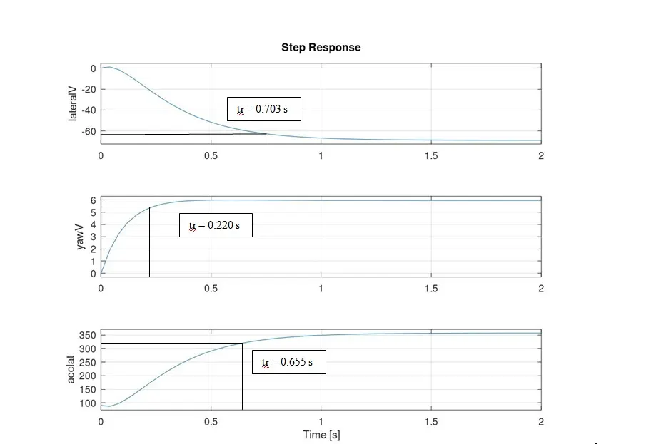
4) Rise time calculation from the step response plot:

3. Plot responses:

1) Passenger Car:

a) Step response:

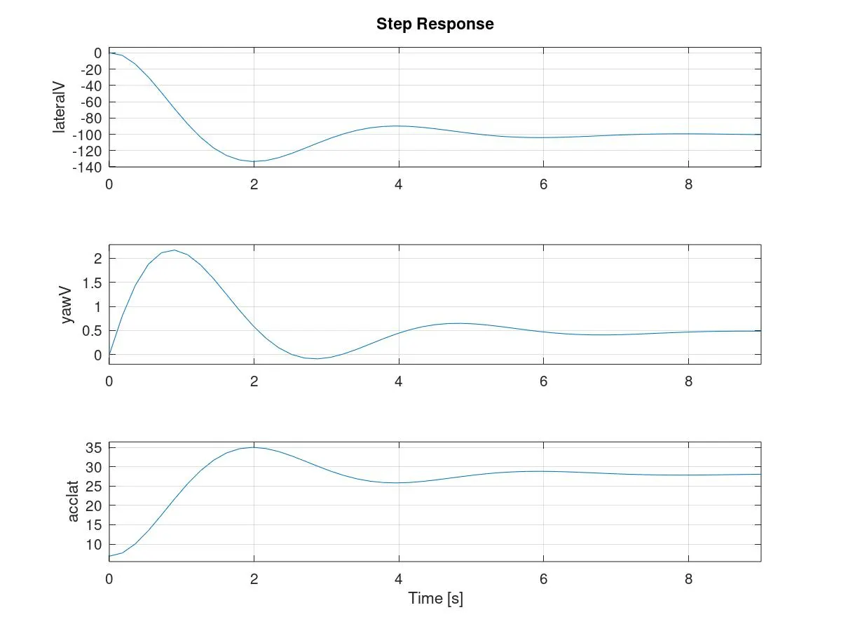
• The step response given to the system and their corresponding sine responses for the passenger car can be co-related using the above graphs.

b) Sine response:

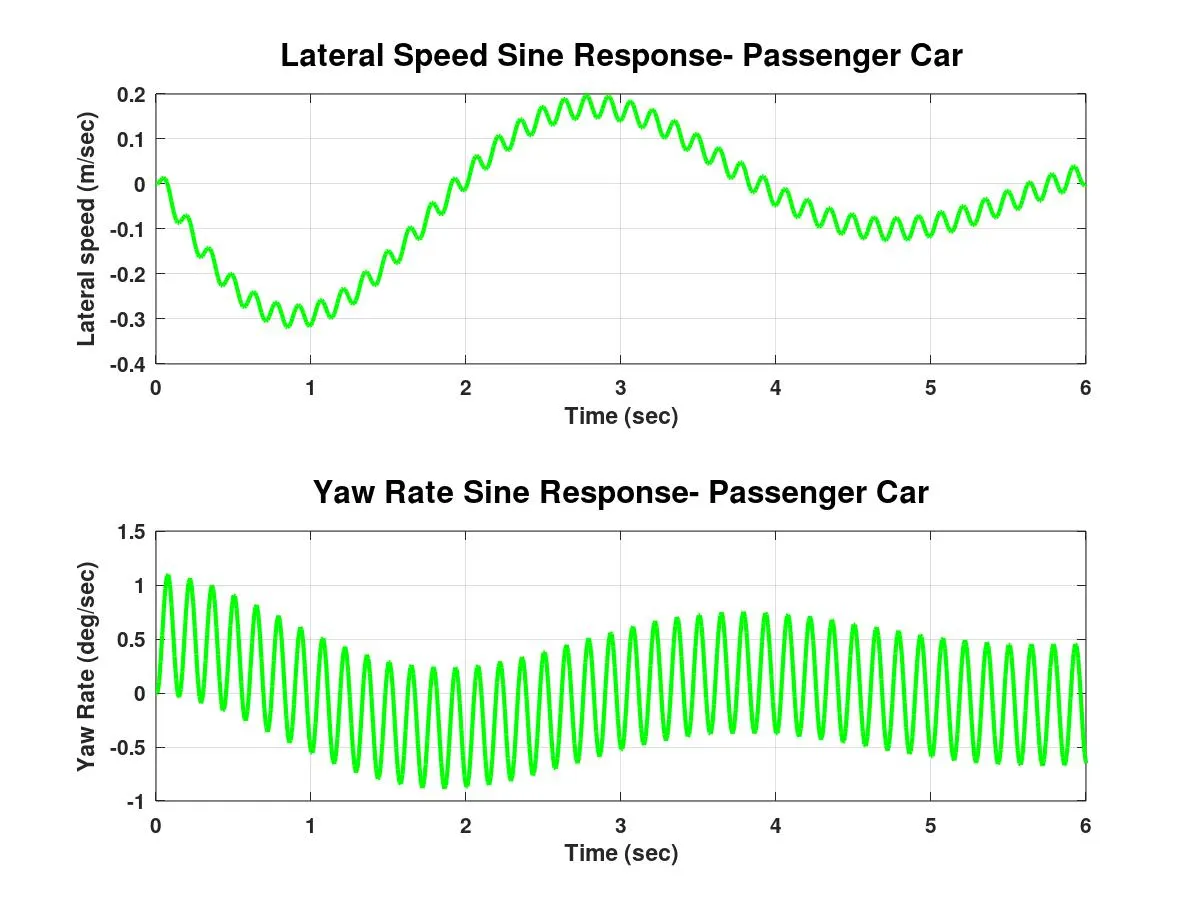
• Yaw Rate Sine vs Step Response: As for the passenger car, the steady-state yaw response is close to 0.5 °/sec which corresponds to the sine response of yaw rate.

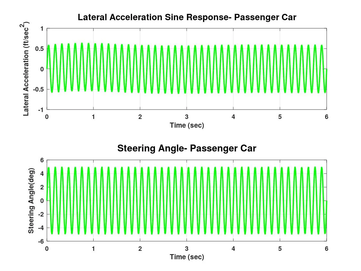
• For 5°, 7 Hz. sine input was given as the steering angle input which co-relates to the response obtained in the 'Steering Angle- Passenger Car' plot where the peak steer angle is 5°.
• Lateral Acceleration Sine vs Step Response: The step response calculated for the passenger car after converting the value to radians is close to 0.48 ft/sec2 which corresponds to the magnitude of sine response of the lateral acceleration plot.

c) Frequency response plot:

1) Yaw Rate frequency response:

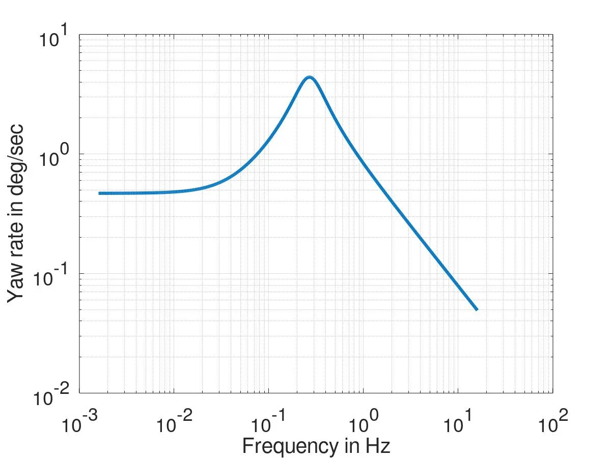
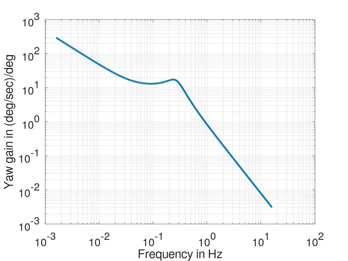
2)Yaw gain frequency response:

2) F1 Car:

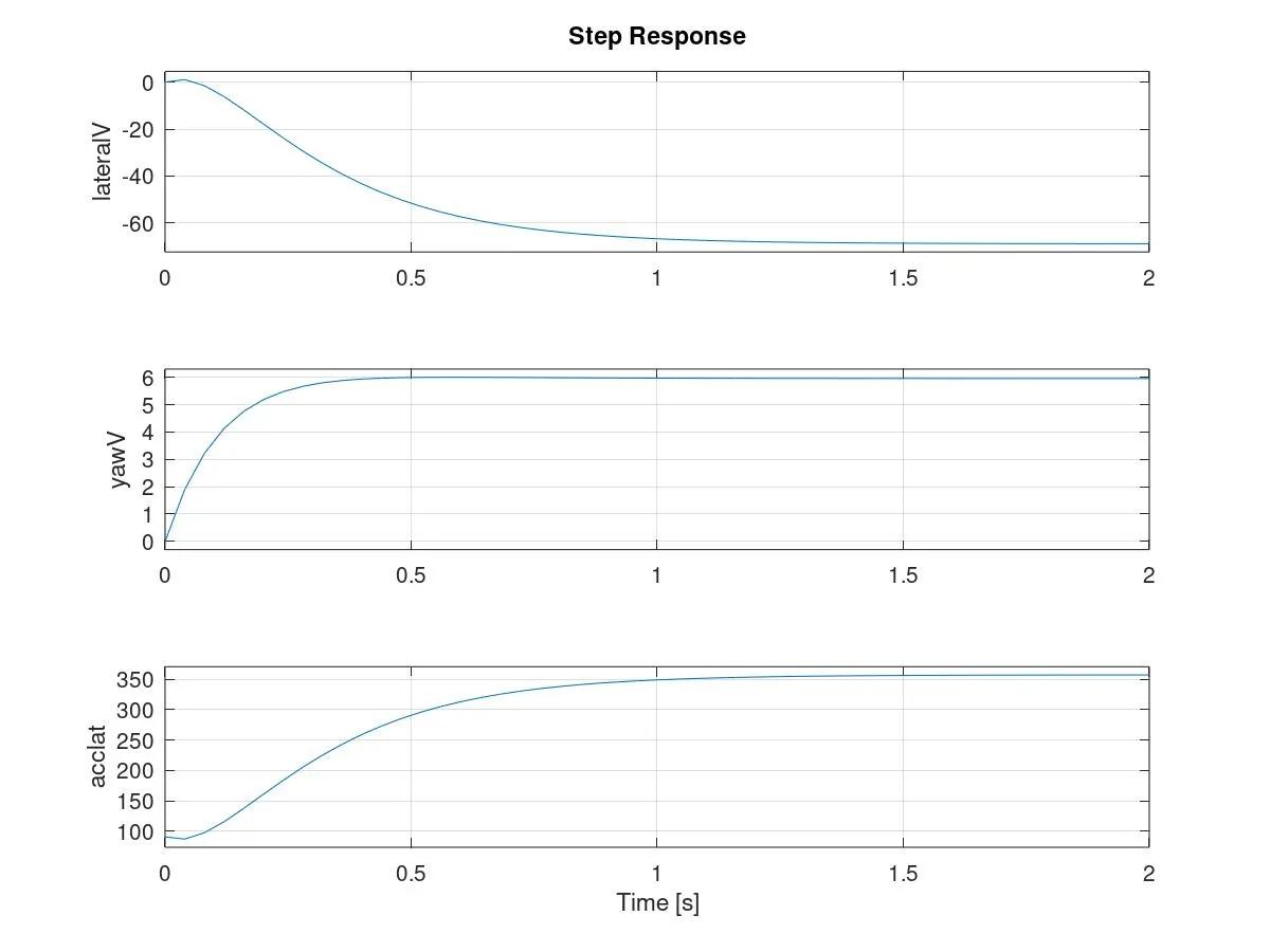
a) Step response:

b) Sine response:

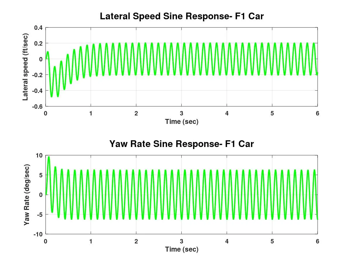
• Yaw Rate Sine v/s Step Response: As can be seen above, the steady state value of the yaw step response is around 6 deg/sec which is the same as sine response for yaw rate.
• Lateral Acceleration Sine v/s Step Response: Since the step response is in radians it needs to be converted to degrees to co-relate with the corresponding sine response. After conversion the step response comes to be around 6.10 ft/sec2 which is the same as the sine response of lateral acceleration

• For 5°, 7 Hz. sine input was given as the steering angle input which co-relates to the response obtained in the 'Steering Angle- F1 Car' plot where the peak steer angle is 5°.

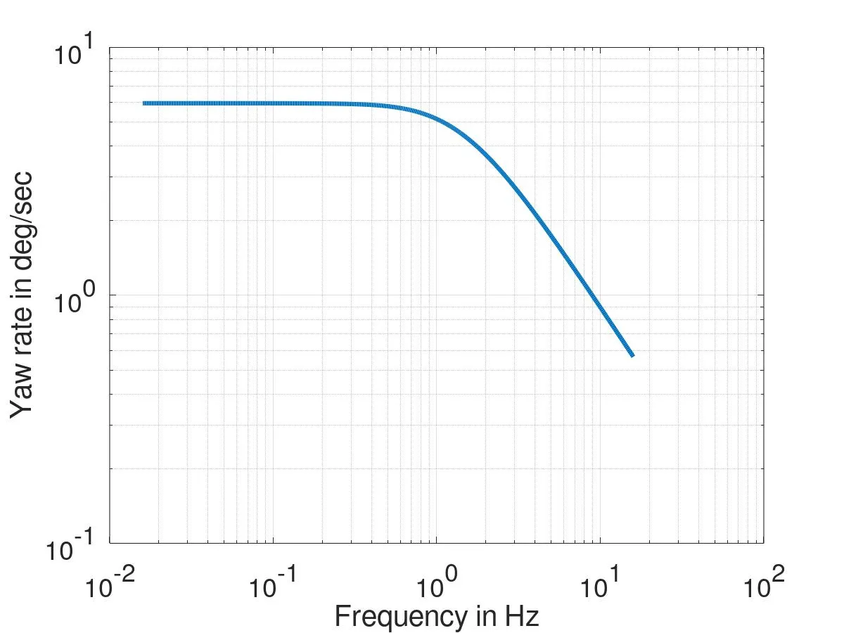
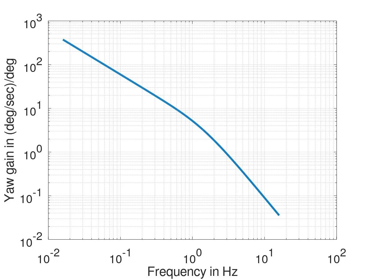
c) Frequency response plot:

1) Yaw Rate frequency response:

2)Yaw gain frequency response:

Conclusion from the response plots:

• The under-damped step response for passenger car is unstable and has a greater overshoot and steady state value compared to an over-damped F1 Car. The response times are larger as a result when compared to the quick responding F1 car.
• The frequency response plot for passenger car show steep increase in the yaw rate while F1 car plot has a smooth increase in yaw.
• As stated previously the sine responses are used as a check plot to make sure the step response makes sense.

5.

Four Wheel Steer: An All Wheel Steer or Four Wheel-Steer vehicle is capable of steering with all the 4 wheels. The main purpose of implementing such a setup is to reduce the turning radius that would let the vehicle easily get through tight spaces. It is often termed as virtual wheel-base system as it mimics a shorter wheel based car’s turning characteristics.

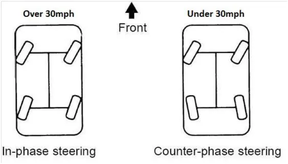
With an In-Phase 4WS rear wheel lag during high-speed turning can also be reduced which will lead to a quicker vehicle response. There are two modes of 4WS:

In-Phase Turn: At high speed, turning the rear wheels through an angle opposite to front wheels might lead to vehicle instability and is thus avoided. Another driving manoeuvre that frequently becomes cumbersome and even dangerous is changing lanes at fairly high speeds. Although this is less steering intensive, this does not require a lot concentration from the driver since he has to judge the space and vehicles behind him. Crab Mode or in-phase turn simplifies this action by letting the rear wheels turn along the same direction as front wheels. This makes the vehicle skid across like a crab more than turn to the next lane.

Counter-Phase Turn: At Slow Speeds rear wheels turn in direction opposite to that of front wheels. This mode is used for navigating through winding slow speed corners and in congested city streets and nooks where better cornering is required for U-turn and tight streets with low speed small turning circle capacities.

For Steady State Yaw gain, r is constant, thus, dr/dt = 0

Taking this initial condition, the equation for FWS becomes:

r= -A^-1 *B*δf

`[[vss],[rss]] = (−1 / det(|A|)) [[(–Cαf⋅a^2-Cαr⋅b^2)/(Izz⋅u),u-(b⋅Cαr-a⋅Cαf)/(m⋅u)],[(a⋅Cαf-b⋅Cαr)/(Izz⋅u),-(Cαf+Cαr)/(m⋅u)]] [[(Cαf)/(ma)],[(α⋅Cαf)/(Izz)]] . [δf]`

Solving this equation gives,

`[[rss],[δf]] = |((L⋅Cαf⋅Cαr)/(det(A)⋅m⋅Izz⋅u))|`

Matlab code for 4 Wheel steering using the bicycle model:

%Four Wheel Steering simulation using bicycle model for an F1 car

a =  5.71*12*25.4*0.001; %Distance between CG and front axle
L =  9.52*12*25.4*0.001; %Wheel Base
m =  1719*0.453592; %mass (kg)
Iz = 865; %yaw moment of inertia (kg-m/s^2)
Caf = 62228*0.453592*9.81; %cornering stiffnes-front axle (N/rad)
Car = 96608*0.453592*9.81; %cornering stiffness- rear axle (N/rad)

%Four Wheel Steering simulation using bicycle model for a Passenger car
%a =  2.92*12*25.4*0.001; %Distance between CG and front axle
%L =  8.33*12*25.4*0.001; %Wheel Base
%m =  2000*0.453592; %mass (kg)
%Iz = 1128; %yaw moment of inertia (kg-m/s^2)
%Caf = 13752*0.453592*9.81; %cornering stiffnes-front axle (N/rad)
%Car = 11460*0.453592*9.81; %cornering stiffness- rear axle (N/rad)

u0=20; %m/s 
g=9.81;%m/s^2

b=L-a; %Distance of CG from rear axle


A=[0, 1, u0, 0; 
  0, -(Caf+Car)/(m*u0), 0, ((b*Car-a*Caf)/(m*u0))-u0;
  0, 0, 0, 1; 
  0, (b*Car-a*Caf)/(Iz*u0), 0, -(a*a*Caf+b*b*Car)/(Iz*u0)]; %System Matrix

B_fws=[0; Caf/m; 0; a*Caf/Iz]; %Input matrix for FWS
B_rws=[0; Car/m; 0; -b*Car/Iz];%Input Matrix for RWS

C_r=[0,0,0,1]; %Output Matrix for Yaw Rate
C_v=[0,1,0,0]; %Output Matrix for Lateral Speed
C_acc=A(2,:)+u0*[0,0,0,1]; %Output Matrix for Lateral Acceleration

%Bode Plots
w = logspace(-1,2,50);

%Defining 6 systems for yaw rate,lat speed and lat acc for FWS and RWS
sys1=ss(A,B_fws,C_r); %Yaw Rate for FWS
sys2=ss(A,B_rws,C_r); %Yaw Rate for RWS
sys3=ss(A,B_fws,C_v); %Lateral Speed for FWS
sys4=ss(A,B_rws,C_v); %Lateral Speed for RWS
sys5=ss(A,B_fws,C_acc,B_fws(2)); %Lateral Acceleration for FWS
sys6=ss(A,B_rws,C_acc,B_rws(2)); %Lateral Acceleration for RWS

[m_fws_r,p_fws_r]=bode(sys1,0,1,w);
[m_rws_r,p_rws_r]=bode(sys2,0,1,w);
[m_fws_v,p_fws_v]=bode(sys3,0,1,w);
[m_rws_v,p_rws_v]=bode(sys4,0,1,w);
[m_fws_acc,p_fws_acc]=bode(sys5,1,w);
[m_rws_acc,p_rws_acc]=bode(sys6,1,w);

figure(1)
subplot(211) 
loglog(w,m_fws_r,'linewidth',2,w,m_rws_r,'-','linewidth',2);
xlabel('Freq (rad/sec)','fontsize',14,'fontweight','bold'); 
title('Yaw rate gain','fontsize',14,'fontweight','bold')
legend('FWS','RWS','location','northeast')
hold on

subplot(212)
semilogx(w,p_fws_r,'linewidth',2,w,(p_rws_r - 180),'-','linewidth',2)
xlabel('Freq (rad/sec)','fontsize',14,'fontweight','bold'); 
title('Yaw Rate phase (deg)','fontsize',14,'fontweight','bold');
legend('FWS','RWS')
hold on

figure(2)
subplot(221)
loglog(w,m_fws_v,'linewidth',2,w,m_rws_v,'-','linewidth',2);
xlabel('Freq (rad/sec)','fontsize',14,'fontweight','bold'); 
title('Lateral Speed Gain','fontsize',14,'fontweight','bold')
legend('FWS','RWS','location','northeast')
hold on

subplot(222)
semilogx(w,p_fws_v-180,'linewidth',2,w,p_rws_v,'-','linewidth',2)
xlabel('Freq (rad/sec)','fontsize',14,'fontweight','bold'); 
title('Lateral Speed phase (deg)','fontsize',14,'fontweight','bold');
legend('FWS','RWS','location','west')

subplot(223)
loglog(w,m_fws_acc,'linewidth',2,w,m_rws_acc,'-','linewidth',2);
xlabel('Freq (rad/sec)','fontsize',14,'fontweight','bold'); 
title('Lateral Acceleration Gain','fontsize',14,'fontweight','bold')
legend('FWS','RWS')

subplot(224)
semilogx(w,p_fws_acc,'linewidth',2,w,p_rws_acc-180,'-','linewidth',2)
xlabel('Freq (rad/sec)','fontsize',14,'fontweight','bold');
title('Lateral acc phase (deg)','fontsize',14,'fontweight','bold');
legend('FWS','RWS','location','west')

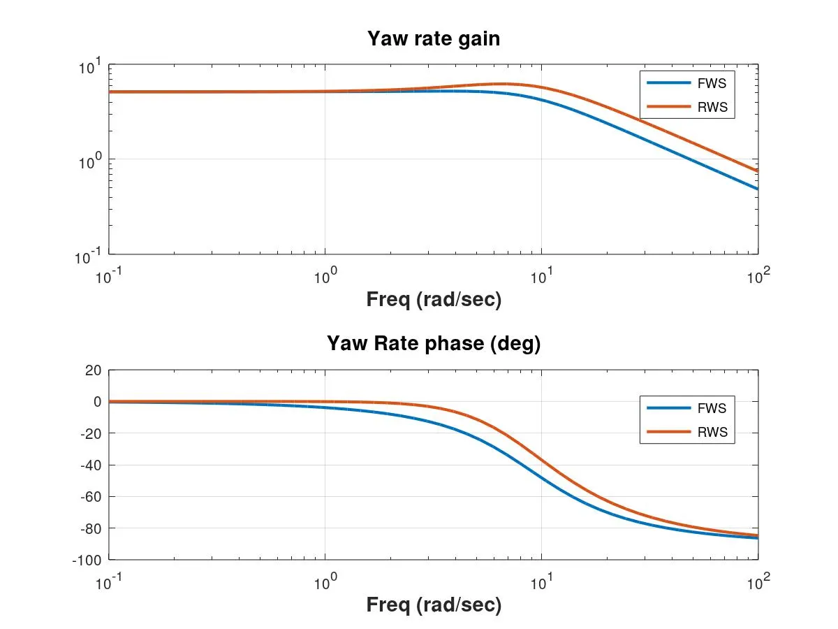
The steady-state yaw gain can be calculated using the above equations:

a) Passenger Car:

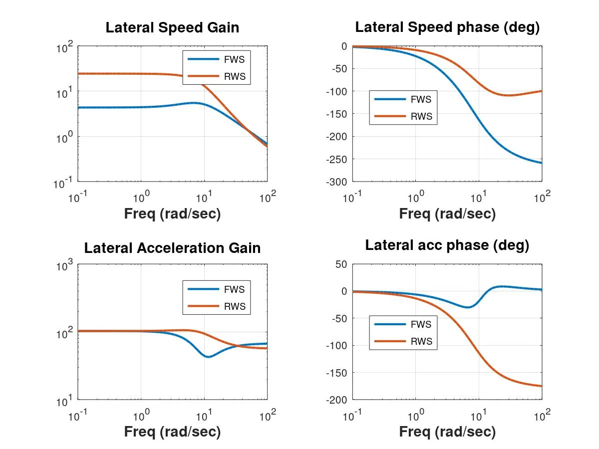
Lateral Speed and Lateral Acceleration are out of phase for FWS and RWS. The phase difference for lateral speed between FWS and RWS is 150°. The gain plot for lateral acceleration highlights the characteristic of RWS where there is a non minimum phase response meaning that instead of reacting in the direction of steering input, the rear wheels may turn in the opposite direction before stabilising and responding to the intended direction. The phase plot shows that the lateral acceleration for FWS and RWS are out of phase by 180° which can lead to stability issues.

b) F1 Car:

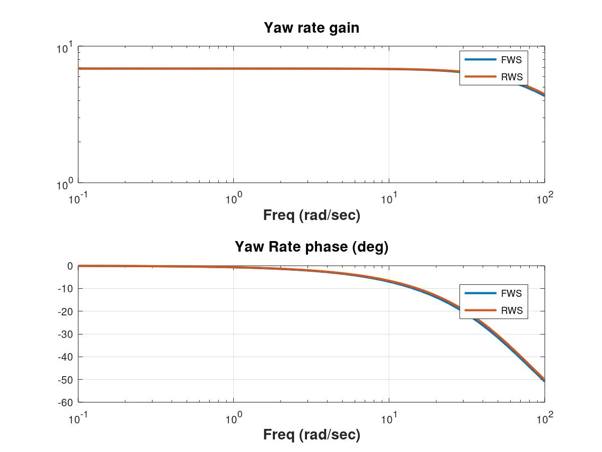
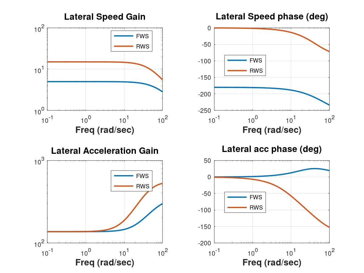
Lateral Speed and Lateral Acceleration are out of phase for FWS and RWS. The phase difference for lateral speed between FWS and RWS is 160°. For the F1 car, the gain plots highlight a different characteristic of RWS where there is a significant gain in RWS lateral speed and acceleration over FWS and the plots dont meet at a single point. The phase plot shows that the lateral acceleration for FWS and RWS are out of phase by 180° which can lead to stability issues.

Drive link to report file:

https://drive.google.com/file/d/1yjTZjb8qGiWiLOEmx4CtqfSxnXxAEzgG/view?usp=sharing

Drive link to assignment folder:

https://drive.google.com/drive/folders/1ZNCSSZZosDKvgShjK4_uJyWe1UoHO2X0?usp=sharing