Week - 10 Hyperelastic Material Models
Hyper-elastic material modelling and validation usin un-axial tensile test simulation:
Aim: To build a material model for a hyper-elastic material using data gathered from experimental tensile test and compare the results for a simulation of a tensile test using a dog-bone specimen model with the actual experimental results validating the model.
Analysis Setup:
Material model:
To get realistic results for any analysis using FEA, a good material model for the material is necessary. A material model can have all sorts of data describing the behaviour of the material in different conditions: say different tensile test curves for different strain rates and much more. This helps getting realistic behaviour of the component with the material model in all sorts of situations.
Building a material model requires test data from various experiments conducted in real life to describe the material behaviour in detail. A complex analysis would benefit from a detailed material model, whereas a simpler simulation would not benefit much. The data collected from an experimental test is first cleaned to make sure any unnecessary data points are filtered out to get clear picture. Usually the same test is repeated a number of times to ensure repeatability of the results. This test data is then inserted in the suitable format into a model: say effective stress-strain curve in x-y co-ordinates. A cleaner data with consistence behaviour in the case of a stress strain plot, inconsistent data points should be avoided as it can affect the stability if the simulation having such an material model. A fitted curve with 98%+ accuracy can solve such issues. After matching for the unit system of the analysis, this data can be added to the simple material model to make it more detailed – for example with the use of material model such as MAT24 – linear piecewise material.
A good practice of the material modelling procedure is the validation of the model. By performing simple analysis for which an experimental test can be performed or such data can be acquired, and then comparing the experimental and analysis results gives a good benchmark for the model. In this exercise, we try and replicate such a process.
Hyper-elastic material model:
A hyper-elastic material can be described as a material which is dominantly elastic in nature – material which can stretch elastically that is without permanent deformation ,several times the original length with application of a small force. A good example would be rubber which is used for its elastic nature over a number of applications.
The material models for hyper-elastic materials such as rubber are different than that of elasto-plastic material such as ductile metals. The method for building a model however is similar. MAT77, 27, 128,129 etc. are used to describe a hyper-elastic material for an analysis. Similar to MAT24, a stress-strain curve is input in the model along with the usual material parameters as density and poisson’s ratio in the MAT77-H card, however, the curve data is for engineering stress-strain and not effective stress-strain. This curve is taken by the program and a curve fit is done to it, along with calculation of hyper-elastic constants. A parameter ‘N’ is defined to state the number of constant to solve for from the curve. This parameter essentially defines the degree of polynomial used to fit the input curve-higher the 'N' figure, higher the degree of polynomial, better the curve fit.
These constants can be then used to describe the curve without actually defining it when ‘N’ is kept at ‘0’. These constants can then be used in specific models such as MAT27-mooney-revlin rubber model and MAT77-o- Ogden rubber to find the closest match in a tensile test. When ‘N’ is kept at ‘1’ the hyper-elastic constants that the program calculates from the curve are Mooney-Revlin constants. We can essentially perform a tensile test using these constants in the same MAT77-H card and get the same results as using MAT27.
The hyper-elastic constants which the program calculates while fitting the curve to the input curve data are generated in the ‘d3hsp’ file and can be grabbed from there for definition of the models.
Process:
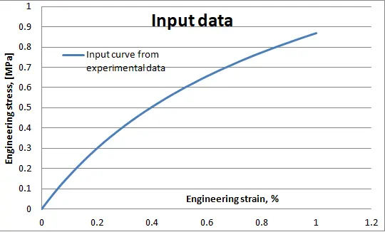
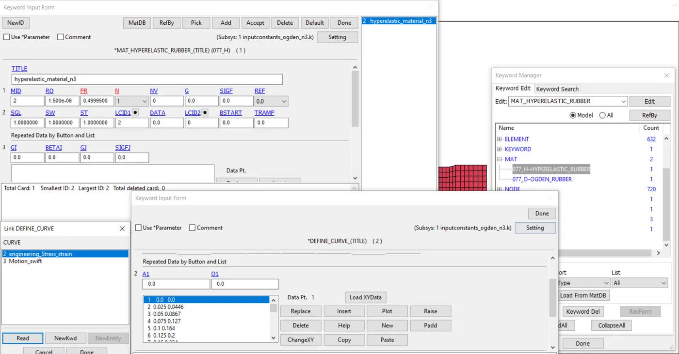
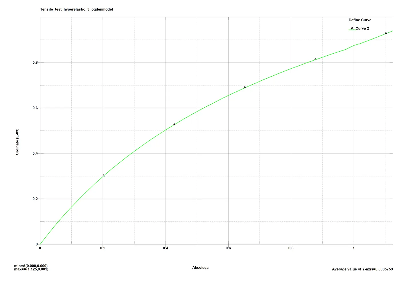
1. Using the engineering stress-strain data provided, a curve is formed and input in the material model using ‘define->curve’ key-wards.
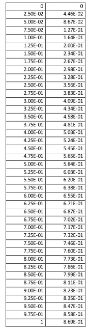
An excel worksheet is maintained with this input curve as well as the simulation results for comparison.
2. A tensile test model is setup for the given dog-bone model, where the boundary conditions are:
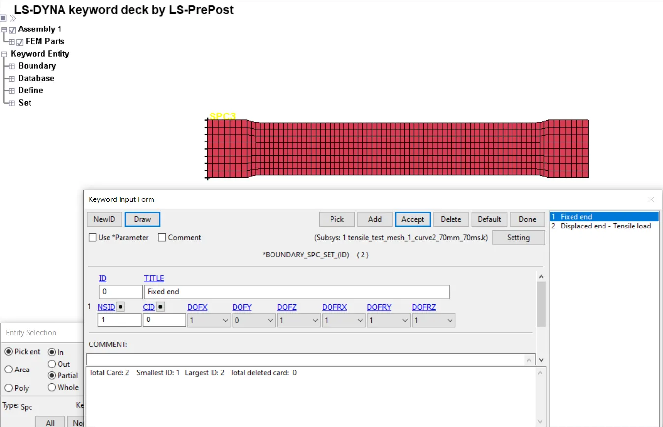
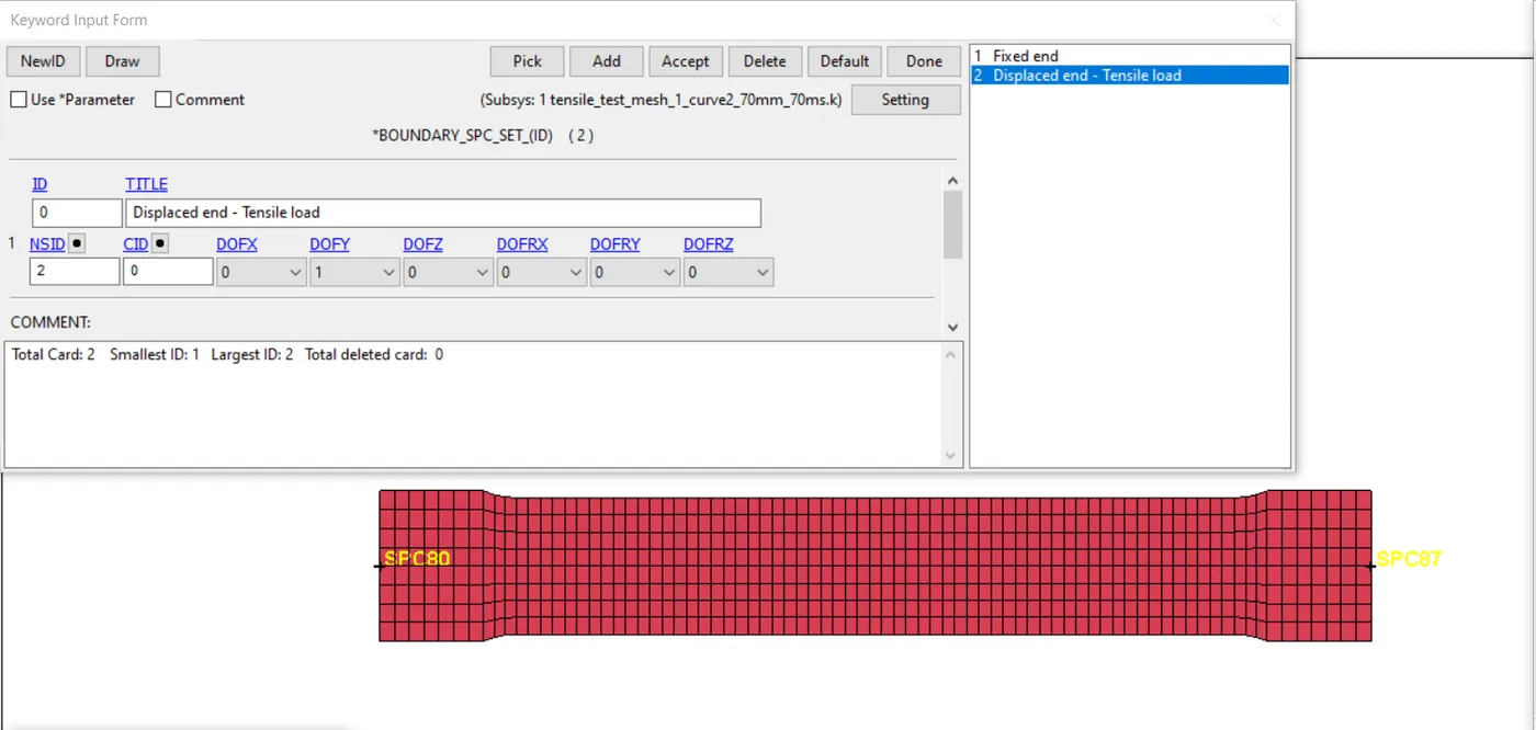
a) One end is fixed with all DOFs locked except translation in lateral direction to allow the compression.
b) All nodes on the other end are added to a node_set to which a ‘prescribed_boundary_condition’ of displacement is applied in the longitudinal axis.
c) The middle node on each of the ends is constrained in all other DOF except translation in the longitudinal axis to avoid contradicting boundary conditions and keep the loading tensile in nature.
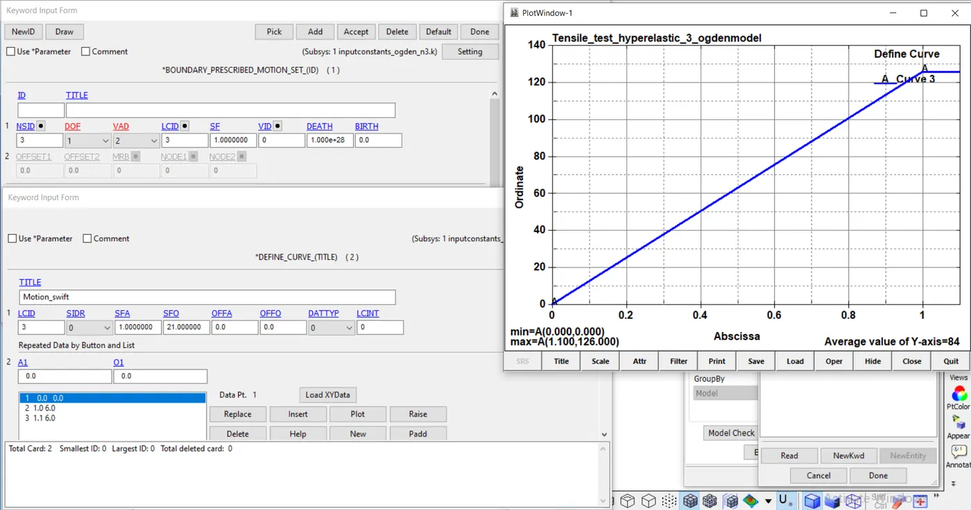
3. A linear displacement curve is defined to get cover the experimental test strain which as stated is 100% - the specimen is stretched to twice its original length.
4. The simulation is performed first only to get the hyper-elastic constants for N=1 through N=3. The fitted curve is tested against the input curve as well. Then these constants are used to define the curve emulating the 3 stages and the results are noted.
5. Finally for the actual simulation for validating the model using the 2 material models mentioned before, the setup is kept the same and the necessary outputs were requested in ‘database’ keyword and the results were compared to the input curves.
6. To understand the process better, implicit analysis is performed.
Procedure:
- Analysis Model and setup:
A dog-bone specimen keyword file with only the mesh data is prepared for the simulation. To keep the analysis simple yet informative, the before mentioned boundary conditions were added along with a MAT77-H material model consisting of the experimental data- the given engineering stress-strain curve using the ‘LCID’ option. As mentioned before, to get a fitted curve and the hyper-elastic parameters, the analysis is run without much tinkering, as the curve fitting is performed before the actual numerical analysis even starts. The constants and the fitted curve data is then retrieved from the ‘d3hsp’ file and gathered in the excel sheet mentioned before.
N=1: Mooney – Rivlin constants:
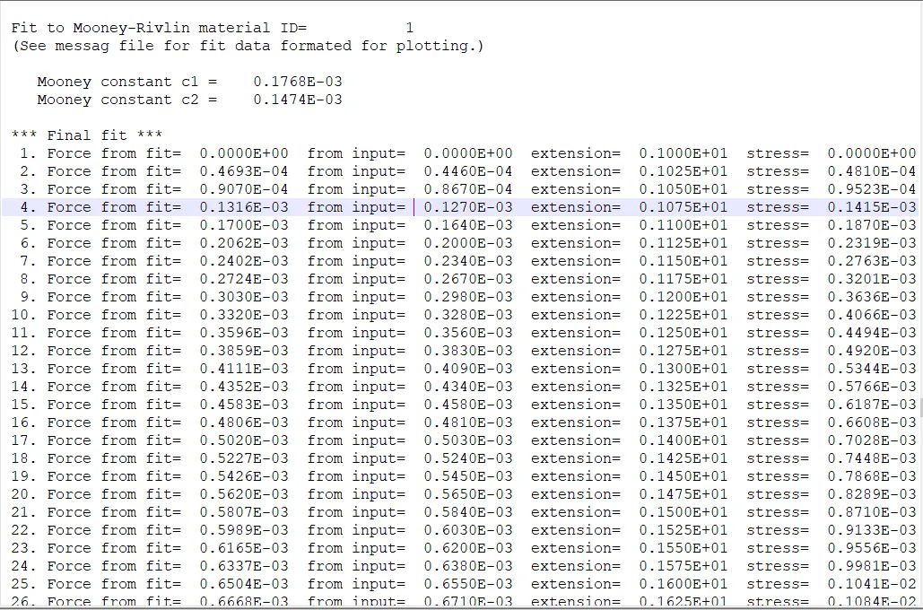
The fitted curve data shows ‘extension’ and ‘stress’ which are the stretch ratio and true stress respectively. For comparison, this data is converted into engineering stress-strain as:
Extension = Stretch ratio = Engineering strain + 1
True stress = Engineering stress * exp(true strain) = engineering stress*ln(1+engineering strain)
|
extension |
True stress[Gpa] |
Engineering strain |
Engineering stress[Gpa] |
|
1.00E+00 |
0.00E+00 |
0.00E+00 |
0.00E+00 |
|
1.03E+00 |
4.81E-05 |
2.50E-02 |
4.69E-05 |
|
1.05E+00 |
9.52E-05 |
5.00E-02 |
9.07E-05 |
|
1.08E+00 |
1.42E-04 |
7.50E-02 |
1.32E-04 |
|
1.10E+00 |
1.87E-04 |
1.00E-01 |
1.70E-04 |
|
1.13E+00 |
2.32E-04 |
1.25E-01 |
2.06E-04 |
|
1.15E+00 |
2.76E-04 |
1.50E-01 |
2.40E-04 |
|
1.18E+00 |
3.20E-04 |
1.75E-01 |
2.72E-04 |
|
1.20E+00 |
3.64E-04 |
2.00E-01 |
3.03E-04 |
|
1.23E+00 |
4.07E-04 |
2.25E-01 |
3.32E-04 |
|
1.25E+00 |
4.49E-04 |
2.50E-01 |
3.60E-04 |
|
1.28E+00 |
4.92E-04 |
2.75E-01 |
3.86E-04 |
|
1.30E+00 |
5.34E-04 |
3.00E-01 |
4.11E-04 |
|
1.33E+00 |
5.77E-04 |
3.25E-01 |
4.35E-04 |
|
1.35E+00 |
6.19E-04 |
3.50E-01 |
4.58E-04 |
|
1.38E+00 |
6.61E-04 |
3.75E-01 |
4.81E-04 |
|
1.40E+00 |
7.03E-04 |
4.00E-01 |
5.02E-04 |
|
1.43E+00 |
7.45E-04 |
4.25E-01 |
5.23E-04 |
|
1.45E+00 |
7.87E-04 |
4.50E-01 |
5.43E-04 |
|
1.48E+00 |
8.29E-04 |
4.75E-01 |
5.62E-04 |
|
1.50E+00 |
8.71E-04 |
5.00E-01 |
5.81E-04 |
|
1.53E+00 |
9.13E-04 |
5.25E-01 |
5.99E-04 |
|
1.55E+00 |
9.56E-04 |
5.50E-01 |
6.17E-04 |
|
1.58E+00 |
9.98E-04 |
5.75E-01 |
6.34E-04 |
|
1.60E+00 |
1.04E-03 |
6.00E-01 |
6.51E-04 |
|
1.63E+00 |
1.08E-03 |
6.25E-01 |
6.67E-04 |
|
1.65E+00 |
1.13E-03 |
6.50E-01 |
6.82E-04 |
|
1.68E+00 |
1.17E-03 |
6.75E-01 |
6.99E-04 |
|
1.70E+00 |
1.21E-03 |
7.00E-01 |
7.14E-04 |
|
1.73E+00 |
1.26E-03 |
7.25E-01 |
7.29E-04 |
|
1.75E+00 |
1.30E-03 |
7.50E-01 |
7.43E-04 |
|
1.78E+00 |
1.35E-03 |
7.75E-01 |
7.58E-04 |
|
1.80E+00 |
1.39E-03 |
8.00E-01 |
7.72E-04 |
|
1.83E+00 |
1.43E-03 |
8.25E-01 |
7.85E-04 |
|
1.85E+00 |
1.48E-03 |
8.50E-01 |
7.99E-04 |
|
1.88E+00 |
1.52E-03 |
8.75E-01 |
8.12E-04 |
|
1.90E+00 |
1.57E-03 |
9.00E-01 |
8.26E-04 |
|
1.93E+00 |
1.61E-03 |
9.25E-01 |
8.38E-04 |
|
1.95E+00 |
1.66E-03 |
9.50E-01 |
8.51E-04 |
|
1.98E+00 |
1.71E-03 |
9.75E-01 |
8.64E-04 |
|
2.00E+00 |
1.75E-03 |
1.00E+00 |
8.77E-04 |
This is repeated for all three cases with N=1 to N=3.
N = 2: Mooney-Rivlin constants:
|
Hyperelastic Constant C10 = 0.2595E-03 |
|
Hyperelastic Constant C01 = 0.4594E-04 |
|
Hyperelastic Constant C11 = - 0.2092E-04 |
|
Hyperelastic Constant C20 = 0.2914E-05 |
|
Hyperelastic Constant C02 = 0.1016E-05 |
|
Hyperelastic Constant C30 = 0.0000E+00 |
Fitted curve data:
|
extension |
True stress[Gpa] |
Engineering strain |
Engineering stress[Gpa] |
|
|
1.00E+00 |
0.00E+00 |
0.00E+00 |
0.00E+00 |
|
|
1.03E+00 |
4.56E-05 |
2.50E-02 |
4.45E-05 |
|
|
1.05E+00 |
9.10E-05 |
5.00E-02 |
8.66E-05 |
|
|
1.08E+00 |
1.36E-04 |
7.50E-02 |
1.27E-04 |
|
|
1.10E+00 |
1.81E-04 |
1.00E-01 |
1.64E-04 |
|
|
1.13E+00 |
2.25E-04 |
1.25E-01 |
2.00E-04 |
|
|
1.15E+00 |
2.70E-04 |
1.50E-01 |
2.34E-04 |
|
|
1.18E+00 |
3.14E-04 |
1.75E-01 |
2.67E-04 |
|
|
1.20E+00 |
3.58E-04 |
2.00E-01 |
2.98E-04 |
|
|
1.23E+00 |
4.01E-04 |
2.25E-01 |
3.28E-04 |
|
|
1.25E+00 |
4.45E-04 |
2.50E-01 |
3.56E-04 |
|
|
1.28E+00 |
4.88E-04 |
2.75E-01 |
3.83E-04 |
|
|
1.30E+00 |
5.32E-04 |
3.00E-01 |
4.09E-04 |
|
|
1.33E+00 |
5.75E-04 |
3.25E-01 |
4.34E-04 |
|
|
1.35E+00 |
6.18E-04 |
3.50E-01 |
4.58E-04 |
|
|
1.38E+00 |
6.61E-04 |
3.75E-01 |
4.81E-04 |
|
|
1.40E+00 |
7.04E-04 |
4.00E-01 |
5.03E-04 |
|
|
1.43E+00 |
7.47E-04 |
4.25E-01 |
5.24E-04 |
|
|
1.45E+00 |
7.90E-04 |
4.50E-01 |
5.45E-04 |
|
|
1.48E+00 |
8.33E-04 |
4.75E-01 |
5.65E-04 |
|
|
1.50E+00 |
8.76E-04 |
5.00E-01 |
5.84E-04 |
|
|
1.53E+00 |
9.19E-04 |
5.25E-01 |
6.03E-04 |
|
|
1.55E+00 |
9.62E-04 |
5.50E-01 |
6.21E-04 |
|
|
1.58E+00 |
1.01E-03 |
5.75E-01 |
6.38E-04 |
|
|
1.60E+00 |
1.05E-03 |
6.00E-01 |
6.55E-04 |
|
|
1.63E+00 |
1.09E-03 |
6.25E-01 |
6.71E-04 |
|
|
1.65E+00 |
1.13E-03 |
6.50E-01 |
6.87E-04 |
|
|
1.68E+00 |
1.18E-03 |
6.75E-01 |
7.02E-04 |
|
|
1.70E+00 |
1.22E-03 |
7.00E-01 |
7.17E-04 |
|
|
1.73E+00 |
1.26E-03 |
7.25E-01 |
7.32E-04 |
|
|
1.75E+00 |
1.31E-03 |
7.50E-01 |
7.46E-04 |
|
|
1.78E+00 |
1.35E-03 |
7.75E-01 |
7.59E-04 |
|
|
1.80E+00 |
1.39E-03 |
8.00E-01 |
7.73E-04 |
|
|
1.83E+00 |
1.44E-03 |
8.25E-01 |
7.86E-04 |
|
|
1.85E+00 |
1.48E-03 |
8.50E-01 |
7.99E-04 |
|
|
1.88E+00 |
1.52E-03 |
8.75E-01 |
8.11E-04 |
|
|
1.90E+00 |
1.56E-03 |
9.00E-01 |
8.23E-04 |
|
|
1.93E+00 |
1.61E-03 |
9.25E-01 |
8.35E-04 |
|
|
1.95E+00 |
1.65E-03 |
9.50E-01 |
8.47E-04 |
|
|
1.98E+00 |
1.70E-03 |
9.75E-01 |
8.58E-04 |
|
|
2.00E+00 |
1.74E-03 |
1.00E+00 |
8.69E-04 |
|
N = 3: Mooney-Rivlin constants:
|
Hyperelastic Constant C10 = 0.2611E-03 |
|
Hyperelastic Constant C01 = 0.4420E-04 |
|
Hyperelastic Constant C11 = -0.6074E-05 |
|
Hyperelastic Constant C20 = -0.2667E-05 |
|
Hyperelastic Constant C02 = -0.9968E-05 |
|
Hyperelastic Constant C30 = 0.1565E-06 |
Fitted curve data:
|
extension |
True stress[Gpa] |
Engineering strain |
Engineering stress[Gpa] |
|
1.00E+00 |
0.00E+00 |
0.00E+00 |
0.00E+00 |
|
1.03E+00 |
4.56E-05 |
2.50E-02 |
4.45E-05 |
|
1.05E+00 |
9.10E-05 |
5.00E-02 |
8.66E-05 |
|
1.08E+00 |
1.36E-04 |
7.50E-02 |
1.27E-04 |
|
1.10E+00 |
1.81E-04 |
1.00E-01 |
1.64E-04 |
|
1.13E+00 |
2.25E-04 |
1.25E-01 |
2.00E-04 |
|
1.15E+00 |
2.70E-04 |
1.50E-01 |
2.34E-04 |
|
1.18E+00 |
3.14E-04 |
1.75E-01 |
2.67E-04 |
|
1.20E+00 |
3.58E-04 |
2.00E-01 |
2.98E-04 |
|
1.23E+00 |
4.01E-04 |
2.25E-01 |
3.28E-04 |
|
1.25E+00 |
4.45E-04 |
2.50E-01 |
3.56E-04 |
|
1.28E+00 |
4.88E-04 |
2.75E-01 |
3.83E-04 |
|
1.30E+00 |
5.32E-04 |
3.00E-01 |
4.09E-04 |
|
1.33E+00 |
5.75E-04 |
3.25E-01 |
4.34E-04 |
|
1.35E+00 |
6.18E-04 |
3.50E-01 |
4.58E-04 |
|
1.38E+00 |
6.61E-04 |
3.75E-01 |
4.81E-04 |
|
1.40E+00 |
7.04E-04 |
4.00E-01 |
5.03E-04 |
|
1.43E+00 |
7.47E-04 |
4.25E-01 |
5.24E-04 |
|
1.45E+00 |
7.90E-04 |
4.50E-01 |
5.45E-04 |
|
1.48E+00 |
8.33E-04 |
4.75E-01 |
5.65E-04 |
|
1.50E+00 |
8.76E-04 |
5.00E-01 |
5.84E-04 |
|
1.53E+00 |
9.19E-04 |
5.25E-01 |
6.03E-04 |
|
1.55E+00 |
9.62E-04 |
5.50E-01 |
6.21E-04 |
|
1.58E+00 |
1.01E-03 |
5.75E-01 |
6.38E-04 |
|
1.60E+00 |
1.05E-03 |
6.00E-01 |
6.55E-04 |
|
1.63E+00 |
1.09E-03 |
6.25E-01 |
6.71E-04 |
|
1.65E+00 |
1.13E-03 |
6.50E-01 |
6.87E-04 |
|
1.68E+00 |
1.18E-03 |
6.75E-01 |
7.02E-04 |
|
1.70E+00 |
1.22E-03 |
7.00E-01 |
7.17E-04 |
|
1.73E+00 |
1.26E-03 |
7.25E-01 |
7.32E-04 |
|
1.75E+00 |
1.31E-03 |
7.50E-01 |
7.46E-04 |
|
1.78E+00 |
1.35E-03 |
7.75E-01 |
7.59E-04 |
|
1.80E+00 |
1.39E-03 |
8.00E-01 |
7.73E-04 |
|
1.83E+00 |
1.44E-03 |
8.25E-01 |
7.86E-04 |
|
1.85E+00 |
1.48E-03 |
8.50E-01 |
7.99E-04 |
|
1.88E+00 |
1.52E-03 |
8.75E-01 |
8.11E-04 |
|
1.90E+00 |
1.56E-03 |
9.00E-01 |
8.23E-04 |
|
1.93E+00 |
1.61E-03 |
9.25E-01 |
8.35E-04 |
|
1.95E+00 |
1.65E-03 |
9.50E-01 |
8.47E-04 |
|
1.98E+00 |
1.70E-03 |
9.75E-01 |
8.58E-04 |
|
2.00E+00 |
1.74E-03 |
1.00E+00 |
8.69E-04 |
The fitted curve-Input curve comparison:
As expected there is virtually no difference in the fitted curves, and little to no deviations.
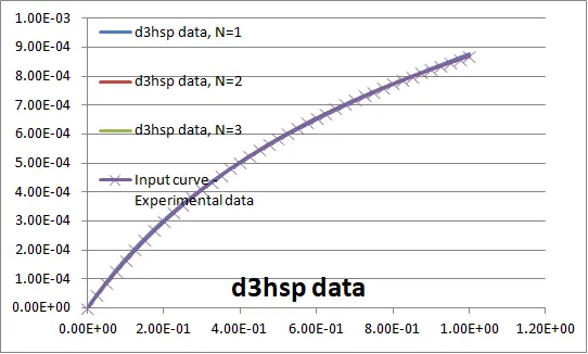
For the actual simulation using these constants in the material models, numerical stability and coverage of experimental data for 100% strain are prioritized. After trying a number of times to get the required results without any instability and unusual results, the following settings were finalised.
1. PART, SECTION, MAT definition:
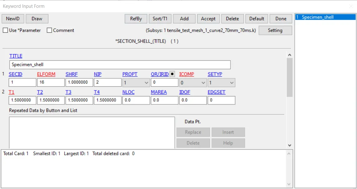
To get a comparative result, the section thickness of the specimen was kept 1.5mm in all the cases with an ‘elform’ of 16 - ‘Fully integrated shell element’ to get most details with more integration points along the thickness.
As mentioned, hyper-elastic natural rubber material properties were used for the MAT77 material card. The engineering stress-strain plot was defined using ‘define->curve’.
Input curve:
- Boundary conditions:
As mentioned above the only boundary conditions defined were the SPCs to make sure the loading is purely tensile, and the prescribed displacement defined with a curve.
a) Fixed end with all DOF constrained except lateral translation:
b) Middle node on each end – free in longitudinal translation, constrained in all other DOFs.
c) Prescribed motion - displacement on the other end for tensile loading:
A liner curve is defined and called upon to impose the boundary condition using a set of nodes the other end from the fixed end.
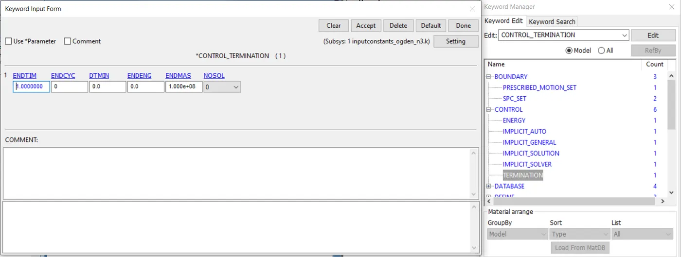
- Database, control settings:
A short end time simulation is finalised as the results gathered are realistic and the computation cost is less.
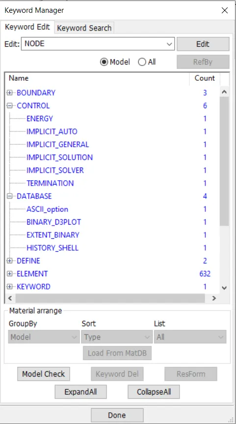
The usual output parameters were requested to get results which can be later compared
Implicit Analysis:
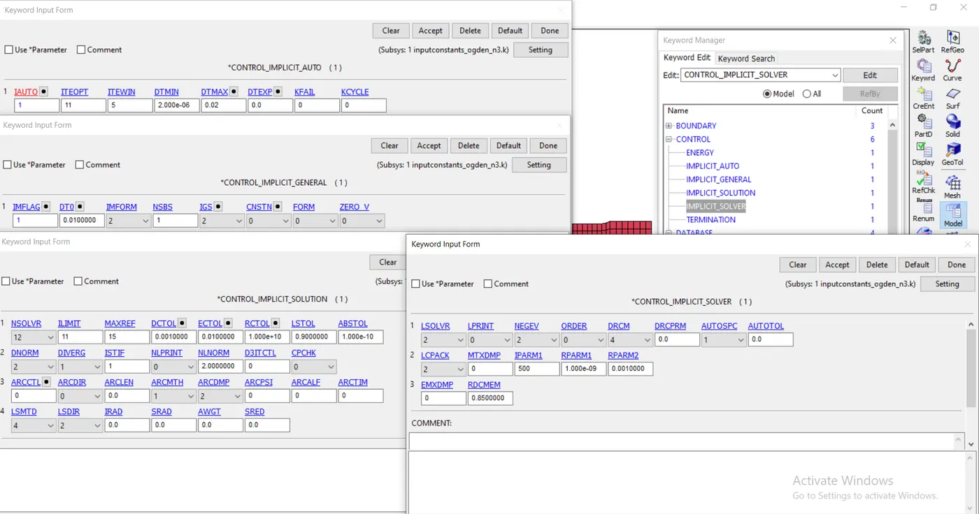
To keep it simple, the run time was to be kept short and was finalised after trying out different iterations. As the implicit analysis requires implicit control cards to be enabled, the default parameters were used for fairness of the results. Only the initial time-step ‘dt0’ and the minimum ‘dtmin’ and maximum ‘dtmax’ time-step parameters were moved around.
Simulation Results:
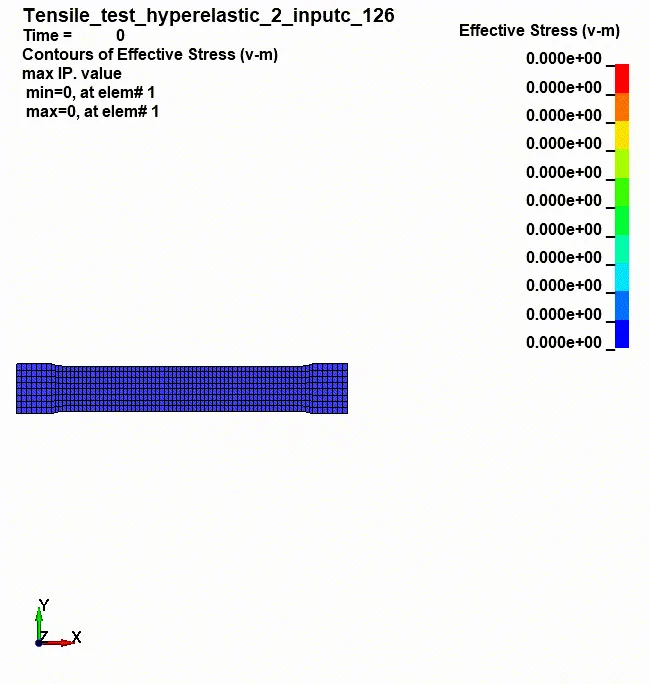
In both the material models, visually the simulation results represent a hyper-elastic material as the stress concentration is observed the corners where the cross section of the specimen reduces. The lateral compression over the same area is observed as well. The middle portion however remains static with almost a constant stress.
- Mooney Rivlin material models:
N = 1:
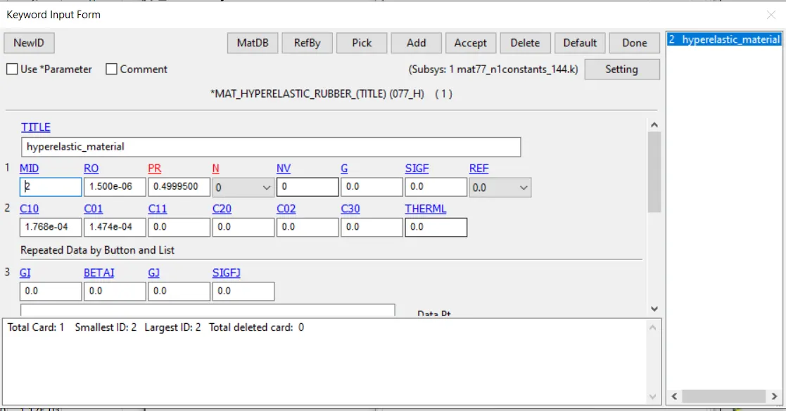
Mooney constant c1 = c10 = 0.1768E-03
Mooney constant c2 = c01 = 0.1474E-03
The mooney-rivlin constant which were calculated previously are used to perform the simulation. The constants define the engineering curve as a result no curve is called upon here, and the ‘N’ is kept at 0.
True stress:
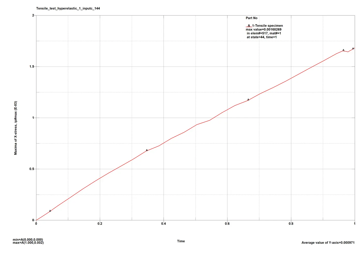
The plot is inconsistent a significant drop at the end is observed. The simulation had some instabilities and some tinkering was required.
True strain:
Comparatively stable and consistent plot is observed due to the linear loading and hyper-elastic nature of the material.
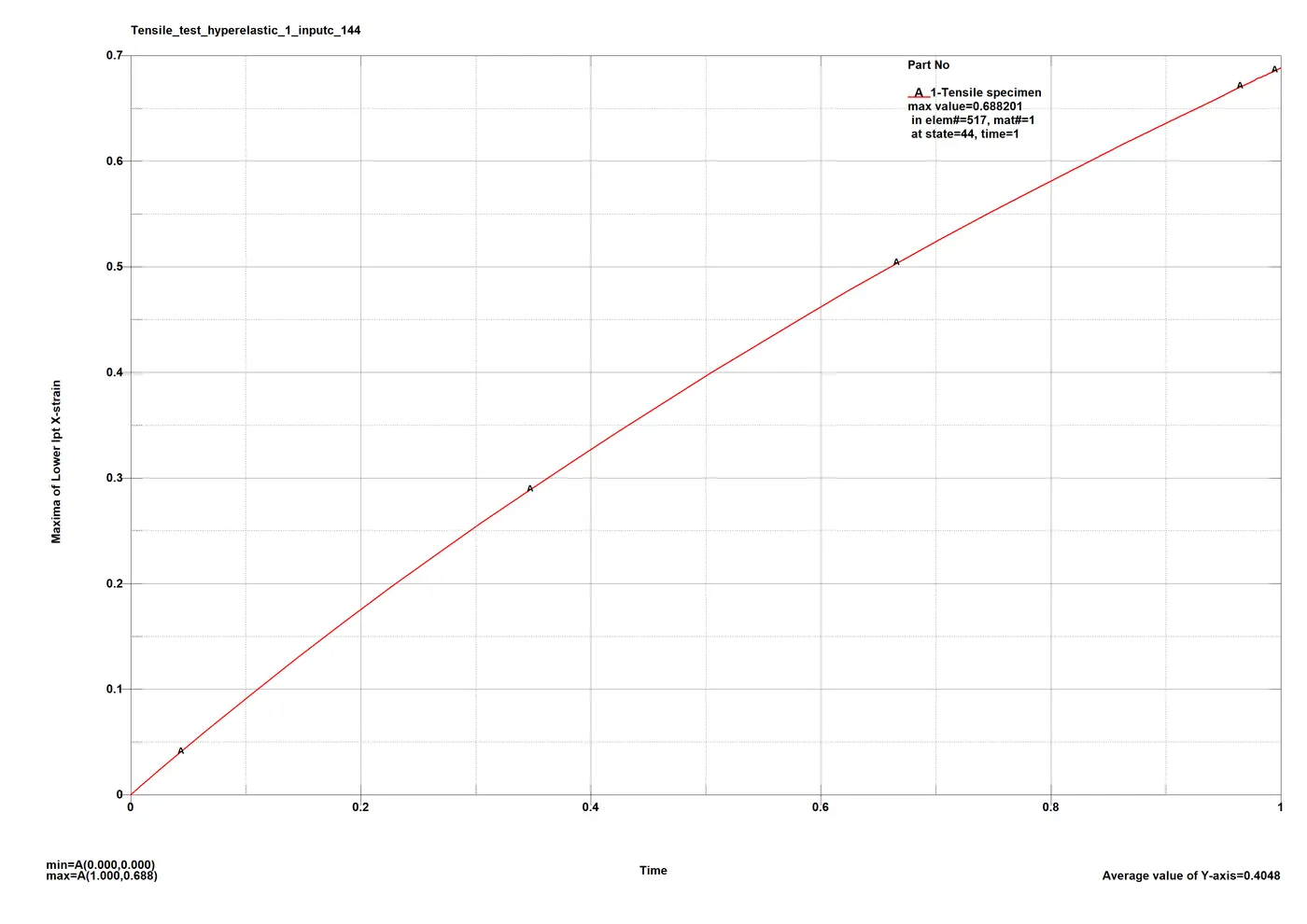
The output results gathered from a simulation are true stress-strains and hence are useless for the purpose of validation. A converted result into engineering output was needed for comparison.
|
Maxima of Lower Ipt X-strain-true strain |
Maxima of X-stress True stress |
Enginering strain |
Engineering stress[Gpa] |
|
|
0.00E+00 |
0.00E+00 |
0.00E+00 |
0.00E+00 |
|
|
9.58E-04 |
1.88E-06 |
9.58E-04 |
1.88E-06 |
|
|
2.47E-03 |
4.86E-06 |
2.48E-03 |
4.85E-06 |
|
|
4.87E-03 |
9.59E-06 |
4.88E-03 |
9.55E-06 |
|
|
8.65E-03 |
1.71E-05 |
8.69E-03 |
1.70E-05 |
|
|
1.46E-02 |
2.93E-05 |
1.47E-02 |
2.89E-05 |
|
|
2.40E-02 |
4.90E-05 |
2.42E-02 |
4.78E-05 |
|
|
3.86E-02 |
8.18E-05 |
3.93E-02 |
7.87E-05 |
|
|
6.14E-02 |
1.38E-04 |
6.33E-02 |
1.30E-04 |
|
|
9.64E-02 |
2.21E-04 |
1.01E-01 |
2.01E-04 |
|
|
1.31E-01 |
3.04E-04 |
1.40E-01 |
2.67E-04 |
|
|
1.64E-01 |
3.83E-04 |
1.78E-01 |
3.25E-04 |
|
|
1.96E-01 |
4.58E-04 |
2.17E-01 |
3.76E-04 |
|
|
2.27E-01 |
5.28E-04 |
2.55E-01 |
4.20E-04 |
|
|
2.58E-01 |
5.98E-04 |
2.94E-01 |
4.62E-04 |
|
|
2.87E-01 |
6.75E-04 |
3.33E-01 |
5.07E-04 |
|
|
3.16E-01 |
7.26E-04 |
3.72E-01 |
5.29E-04 |
|
|
3.45E-01 |
8.00E-04 |
4.11E-01 |
5.67E-04 |
|
|
3.72E-01 |
8.59E-04 |
4.51E-01 |
5.92E-04 |
|
|
3.99E-01 |
9.34E-04 |
4.91E-01 |
6.26E-04 |
|
|
4.26E-01 |
9.75E-04 |
5.30E-01 |
6.37E-04 |
|
|
4.52E-01 |
1.05E-03 |
5.71E-01 |
6.70E-04 |
|
|
4.77E-01 |
1.12E-03 |
6.12E-01 |
6.95E-04 |
|
|
5.02E-01 |
1.17E-03 |
6.51E-01 |
7.08E-04 |
|
|
5.26E-01 |
1.24E-03 |
6.92E-01 |
7.31E-04 |
|
|
5.49E-01 |
1.29E-03 |
7.32E-01 |
7.48E-04 |
|
|
5.72E-01 |
1.36E-03 |
7.71E-01 |
7.66E-04 |
|
|
5.94E-01 |
1.42E-03 |
8.11E-01 |
7.86E-04 |
|
|
6.16E-01 |
1.49E-03 |
8.52E-01 |
8.06E-04 |
|
|
6.37E-01 |
1.56E-03 |
8.91E-01 |
8.24E-04 |
|
|
6.58E-01 |
1.63E-03 |
9.31E-01 |
8.42E-04 |
|
|
6.69E-01 |
1.65E-03 |
9.52E-01 |
8.47E-04 |
|
|
6.74E-01 |
1.65E-03 |
9.62E-01 |
8.41E-04 |
|
|
0.676560283 |
0.001645245 |
0.967099815 |
8.36E-04 |
|
|
6.78E-01 |
0.001645413 |
0.970541949 |
8.35E-04 |
|
|
6.79E-01 |
0.001650125 |
0.972355443 |
8.37E-04 |
|
|
6.81E-01 |
0.001655219 |
0.975194479 |
8.38E-04 |
|
|
6.82E-01 |
0.00165888 |
0.977226851 |
8.39E-04 |
|
|
6.83E-01 |
0.001663544 |
0.979729014 |
8.40E-04 |
|
|
6.84E-01 |
0.001667672 |
0.982014124 |
8.41E-04 |
|
|
6.86E-01 |
0.001673114 |
0.984949525 |
8.43E-04 |
|
|
6.87E-01 |
0.001677482 |
0.987295978 |
8.44E-04 |
|
|
6.88E-01 |
0.001682385 |
0.989673666 |
8.46E-04 |
|
|
6.88E-01 |
0.001682691 |
0.990131491 |
8.46E-04 |
|
Comparison for Mooney-Rivlin model:
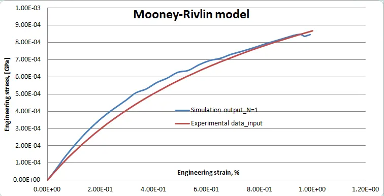
The difference is considerable and as mentioned due to the numerical instability the flaws in the model are amplified. The 2 hyper-elastic (mooney-rivlin) constants definition of experimental input data isn’t detailed enough and as a result there is a consistent error between the plots.
N = 2:
The number of terms defining the input curve increased from 2 in the previous case to 4. This gives betters resolution and better fit which results in closer results.
|
Hyperelastic Constant C10 = 0.2595E-03 |
|
Hyperelastic Constant C01 = 0.4594E-04 |
|
Hyperelastic Constant C11 = - 0.2092E-04 |
|
Hyperelastic Constant C20 = 0.2914E-05 |
|
Hyperelastic Constant C02 = 0.1016E-05 |
|
Hyperelastic Constant C30 = 0.0000E+00 |
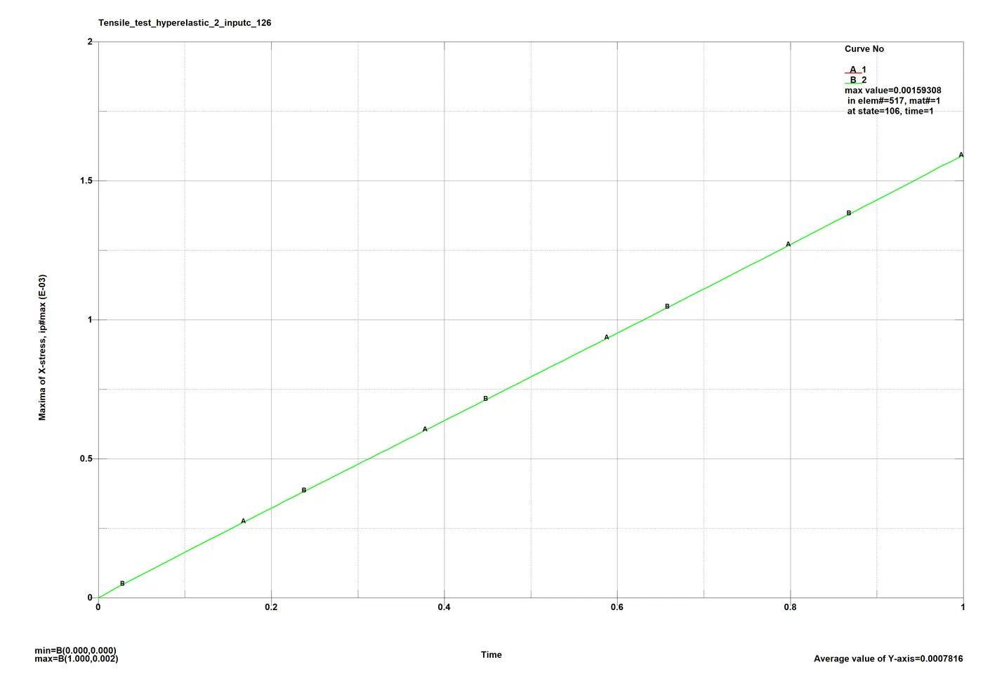
True stress:
The difference is obvious with very consistent and stable output plot compared to previous case.
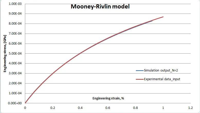
Comparison for Mooney-Rivlin model:
The higher resolution of input makes the fitted curve better, reducing the instabilities and error between the curves. There is hardly any difference between the simulation results and the inputs.
N = 3: With even more constants defining the input plot, the results should be almost identical.
|
Hyperelastic Constant C10 = 0.2611E-03 |
|
Hyperelastic Constant C01 = 0.4420E-04 |
|
Hyperelastic Constant C11 = -0.6074E-05 |
|
Hyperelastic Constant C20 = -0.2667E-05 |
|
Hyperelastic Constant C02 = -0.9968E-05 |
|
Hyperelastic Constant C30 = 0.1565E-06 |
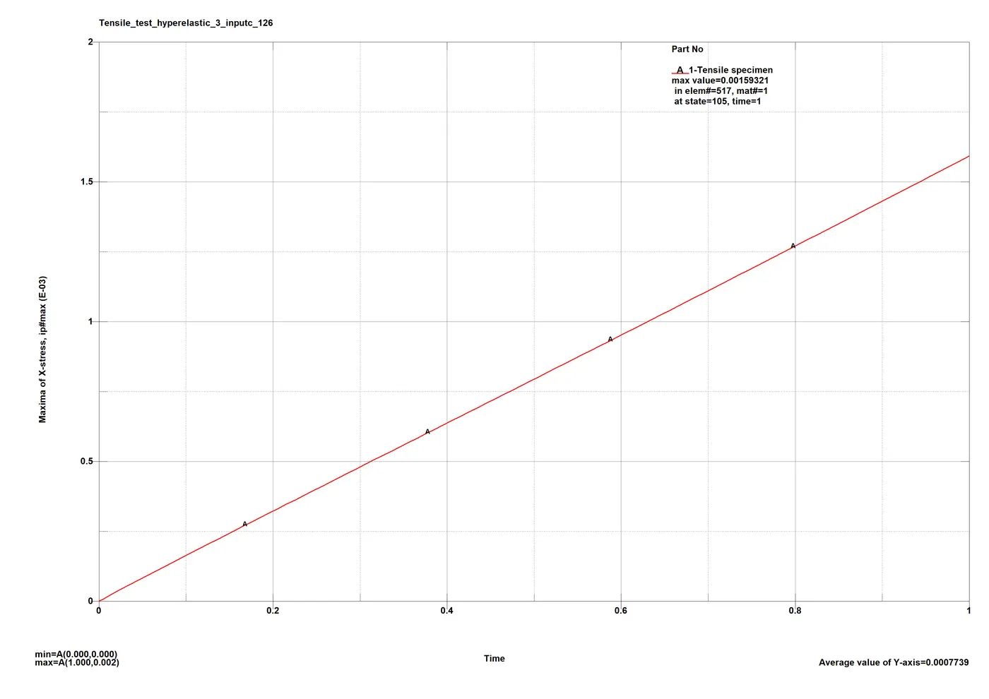
True stress:
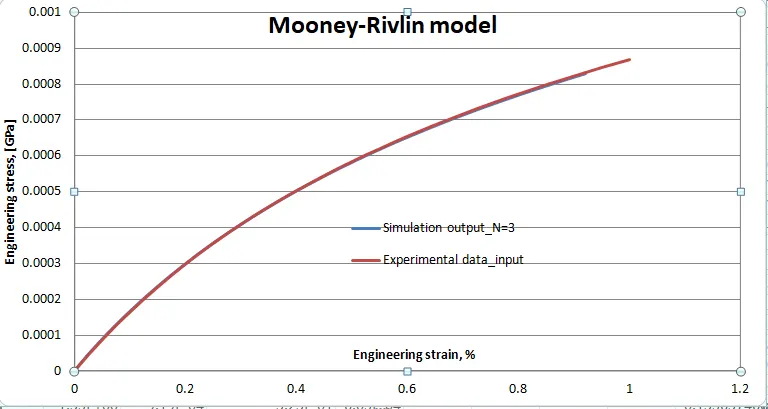
Comparison for Mooney-Rivlin model:
As expected the output plot mimics the input all the way with very small deviations.
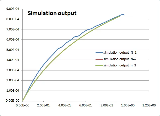
Mooney Rivlin models all cases:
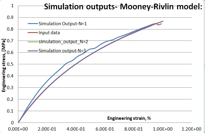
Except the 1st case with ‘N=1’, the other two models perform flawlessly. The error is neglegible and the plots are consistant. The model can be assumed to have satisfactory validation for the test.
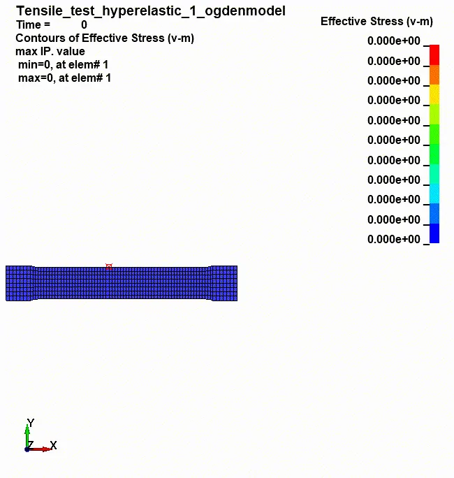
- Ogden material models:
The visual representation of the result is similar to that of the Mooney-RIvlin material model.
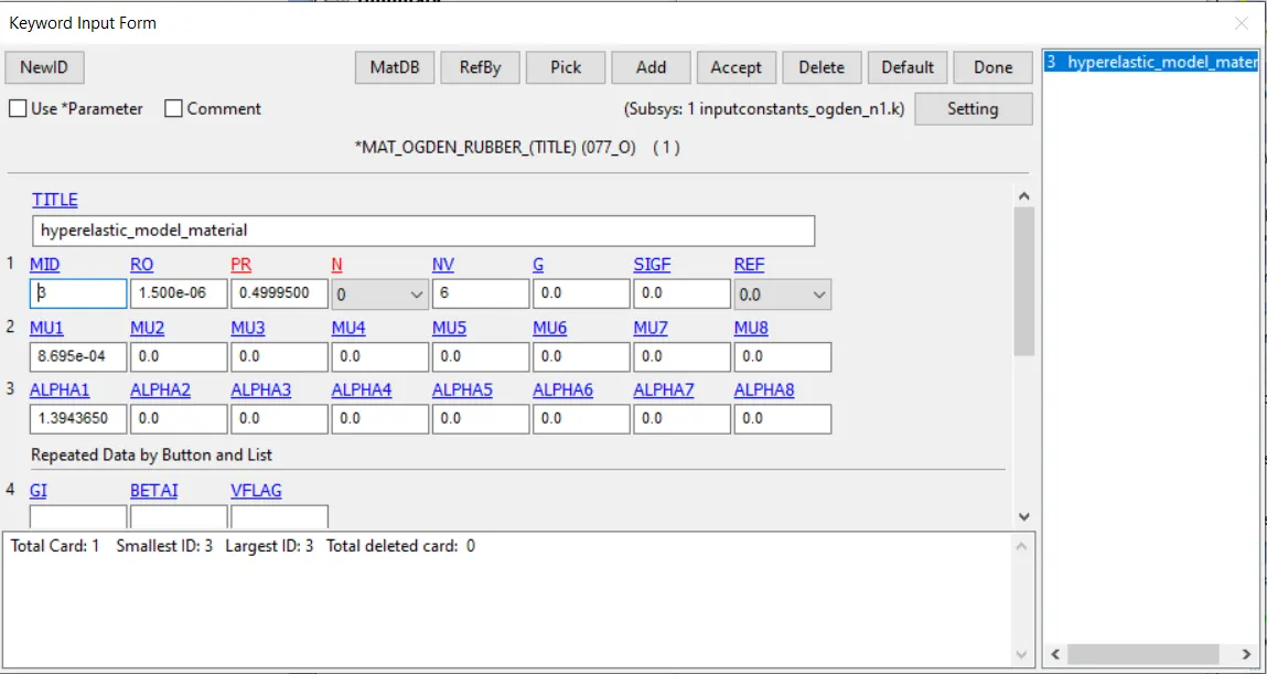
For the 2nd case, using the Ogden rubber model – MAT77-O, the same constants are used for a similar set of curve fitting parameters – ‘mu’ and ‘alpha’.
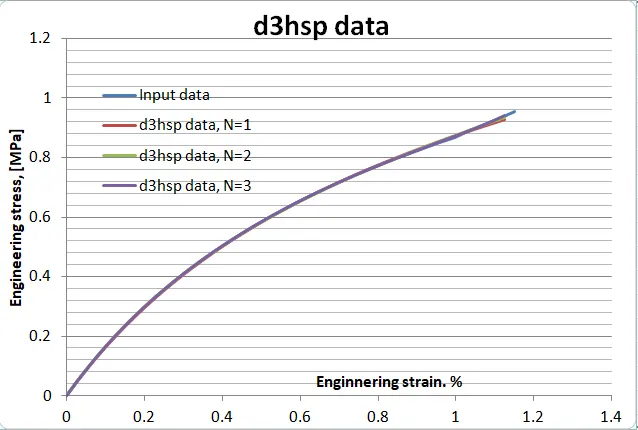
The fitted curve using the same procedure gave similar results, very small deviations and overall an accurate fit across the three cases.
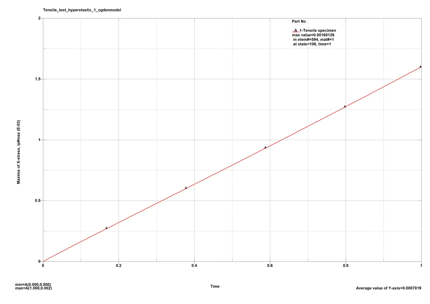
Ogden model, N=1: Lower resolution should have some problems capturing the complete behaviour of the input plot, affecting the simulation results.
|
Final approximate solution |
|
mu(1)= 8.6951487498830E-04 |
|
alpha(1)= 1.3943652230966E+00 |
True stress: compared to mooney-rivlin model, the plot is cleaner and consistent.
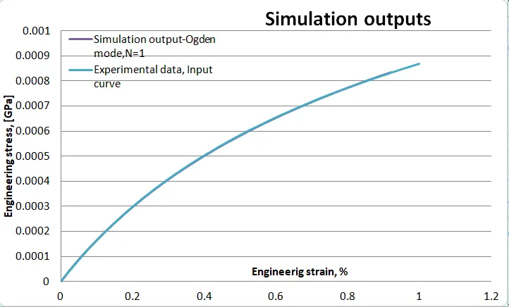
Ogden model, N=1:
As the true stress output suggested, the model mimics the experimental data closely, with very minute deviations.
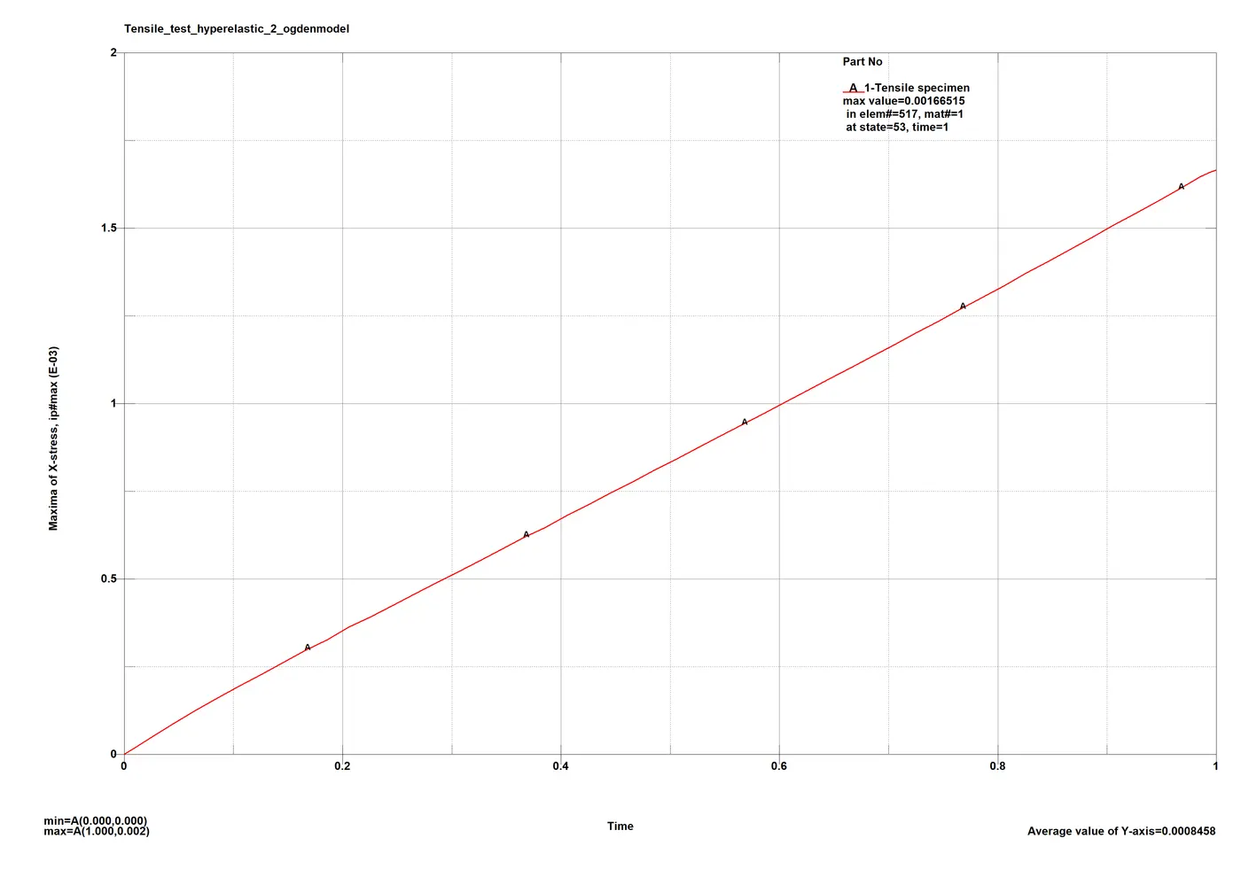
Ogden model-N = 2:
|
mu(1)= |
7.51E-06 |
alpha(1)= |
4.44E+00 |
|
mu(2)= |
1.12E-03 |
alpha(2)= |
1.07E+00 |
True stress:
Slight deviations and inconsistency at the beginning and the end of the analysis can be observed as the behaviour of the plot changes. Low resolution of the data points due to higher time-steps might cause such errors.
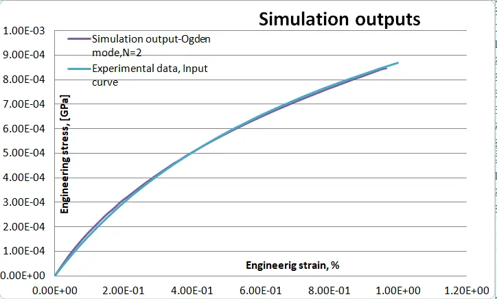
Ogden model, N=2:
The results are repeated in the engineering plots, as there is noticeable difference between the inputs and outputs. As mentioned, higher resolution might change things up but as it is the results can e deemed as satisfactory with the error being minute.
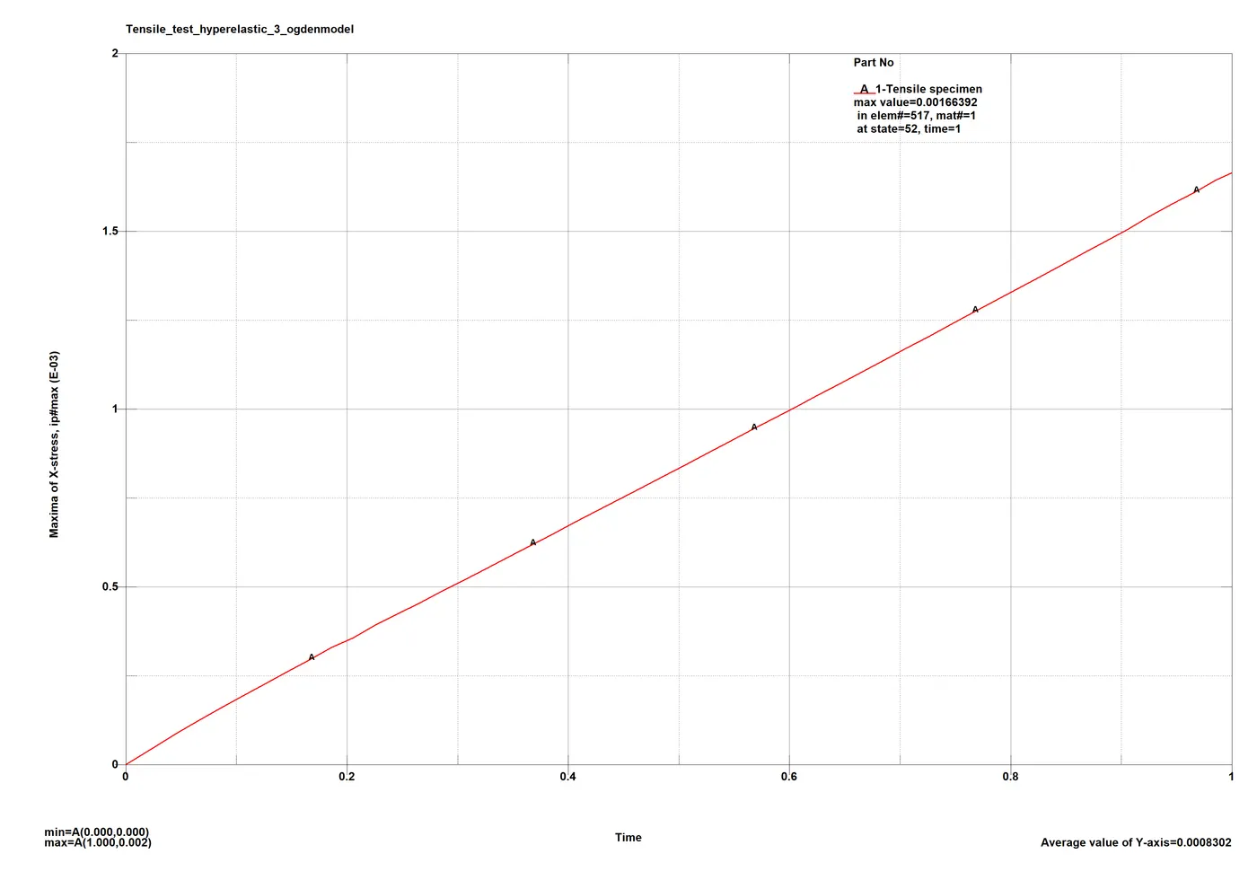
Ogden model-N = 3:
|
approximate solution |
||
|
mu(1)= 3.5623977209387E-13 |
alpha(1)= |
2.48E+01 |
|
mu(2)= 1.5037618729876E-04 |
alpha(2)= |
1.30E+00 |
|
mu(3)= 7.6755709917801E-04 |
alpha(3)= |
1.34E+00 |
True stress:
There is still a slight deviation at the start, with small improvement over the previous case.
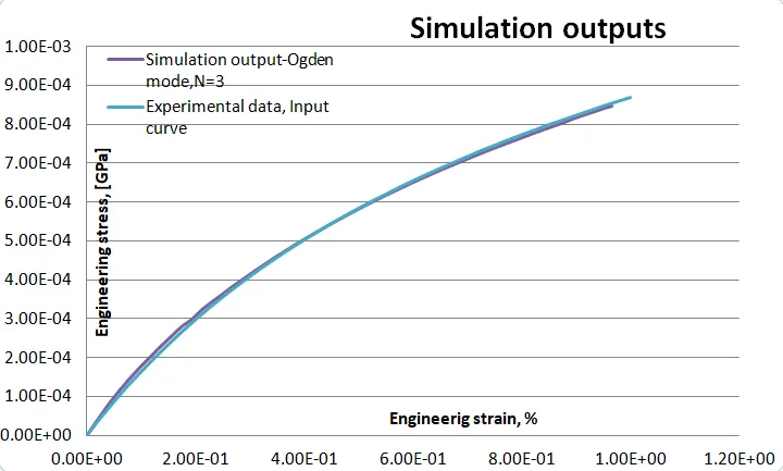
Ogden model, N=3:
The plots appear to have a slight error, but the results are better than the previous case.
Ogden models all cases:
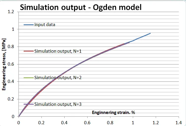
In summary, the ogden material models perform just as good as the mooney-rivlin model, however, the plots are a bit more accurate in the ogden rubber case, and there is less deviation over the 3 cases.
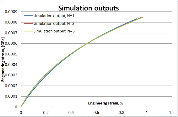
Comparison of the models:
- Both the material models are compatible for the given material – Natural rubber, with very close simulation results to the experimental data. If the 1st case for the ‘Mooney-Rivlin’ material model is neglected, the other two cases perform exceptionally well with little to no errors.
- The numerical instabilities encountered in non-linear implicit analysis might be the differentiating factor for the ogden material model, which causes small inconsistency in the simulation results deviating from the experimental data. The results are still acceptable and the difference of outputs in the two material models it really small.
Conclusion:
- As stated earlier, both the material models are highly compatible for the test material and the simulation results are marginally different. A non-linear implicit analysis is bound to have instabilities and this might have caused the errors. With the error margin being this small, any factor might be responsible hence further testing of the model is necessary to form better conclusions. A bi-axial tensile test in usually preferred for hyper-elastic materials.
- Despite the instabilities, the ‘Mooney-Rivlin’ material model produces exceptional results for ‘N=2’ and ‘N=3’ cases, i.e. with more hyper-elastic constants. On the contrary, ‘Ogden’ material model produces slightly deviated result across all the 3 cases – suggesting the fact that it is not the right material model for the given test material. As stated, the sample space of simulation results is too small for proper validation of the material models and this conclusion is strictly based on the ‘Uni-axial tensile test’ validation.
- A higher degree polynomial should be preferred for curve fitting of experimental data using MAT77-H model – N>1. The non-linear nature of the stress-strain plots for hyper-elastic materials requires it. A thorough validation over a number of tests, with repeatable validation test is necessary to get to a final conclusion especially in hyper-elastic material models.