Week - 8 Mass Scaling

Objective: To study and understand ‘mass scaling’ technique used in explicit analysis and how it affects the time-step and overall simulation time for a given analysis using trial and error method.

Analysis Setup:

In an explicit dynamic analysis, the time step is computed using the stress wave propagation phenomenon. In any contact based analysis, where two bodies collide in space, a stress wave in generated. This wave is initiated at the point of contact and travels throughout the bodies till it gets damped down. The speed with which this wave propagates, is approximately equal to the speed of sound through that material – solid, fluid etc. The speed of sound in a material is proportional to the square root of the ratio of – elastic modulus of the material to the density if the material.

c = `√(E/ρ)`

The time-step, for which the equation of motion is solved to calculate the displacement, and from there strain, stress, acceleration, forces etc. is figured out using this speed and the smallest element length in the given analysis model.

t_step = `l_min/c`

Usually explicit analysis is performed in impact and crash tests. A large quantity of components are involved in such cases, which makes it logical to keep the mesh density on the coarser side. For better accuracy a finer mesh and hence large computation power and computation time would be required. For a complex geometry where mesh refinement is required at stress concentration zones, it is difficult to make the compromise of accuracy and computation capacity. Mass scaling is used in such cases, where to alter the ‘t_step’ instead of increasing the element length, the density of the particular element is increased by adding arbitrary mass to it. This decreases the ‘c’ – speed of stress wave propagation and as a result reduces ‘t_step’.

A good practice would be keeping the added mass as low as possible with a limit of 5% of the original mass. Additional mass increases the Internal energy of the system and may cause instabilities in the simulation.

Analysis setup:

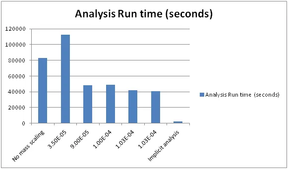
The given case from its parameters is clearly an arbitrary example as the prescribed velocity is too low and what is supposed to be an explicit dynamic analysis has an end time of 600 seconds. This makes the analysis unnecessarily lengthy, and costly. The objective is to monitor the computed ‘analysis time’ for the default settings and observe the changes with respect to mass scaling. In case 1, the given analysis file is run as it is and the analysis time is noted. Keeping the added mass limit in mind, mass scaling is performed iteratively and the respective changes in the analysis run time are noted. A histogram is plotted for all the cases to draw conclusion. The same analysis is then performed using implicit time integration method to note the same.

Mass scaling:

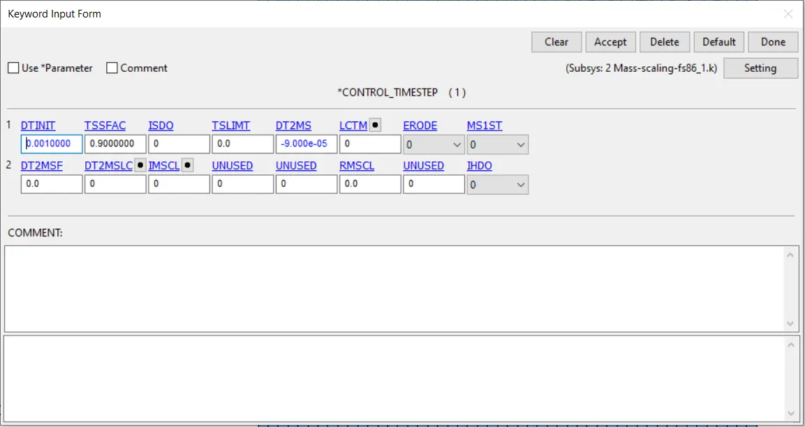
Using the ‘control_Time-step’ keyword, the mass scaling is performed. In the keyword, parameters such as:

‘DTINIT’ – Initial time step,

‘dt2ms’ – Time step size for mass scaled solution – which is the limiting time step – any computed time step below this limit is scaled up to this limit by adding arbitrary mass to the element which requires a smaller time step,

‘TSSFAC’- scale factor for computed time step – effective time step in percentage.

and many such others can be added. In this exercise the ‘dt2ms’ parameter is changed from case to case while keeping the 'tssfac' parameter the same at '0.9'. In a sense, the minimum time step is maintained to a given ‘(dt2ms*tssfac)’ limit using this option while the added mass limit is the final criteria. By increasing the minimum time step by a small amount, the total run time of the analysis is reduced without significantly disturbing the stability and affecting the analysis outcomes.

Procedure:

As mentioned above, the ‘dt2ms’ values are changed for each case. After going on with the analysis, the ‘analysis run time’ is calculated and noted.

Case 1:

Default setup with no mass scaling, as in no ‘control_timestep’ card used.

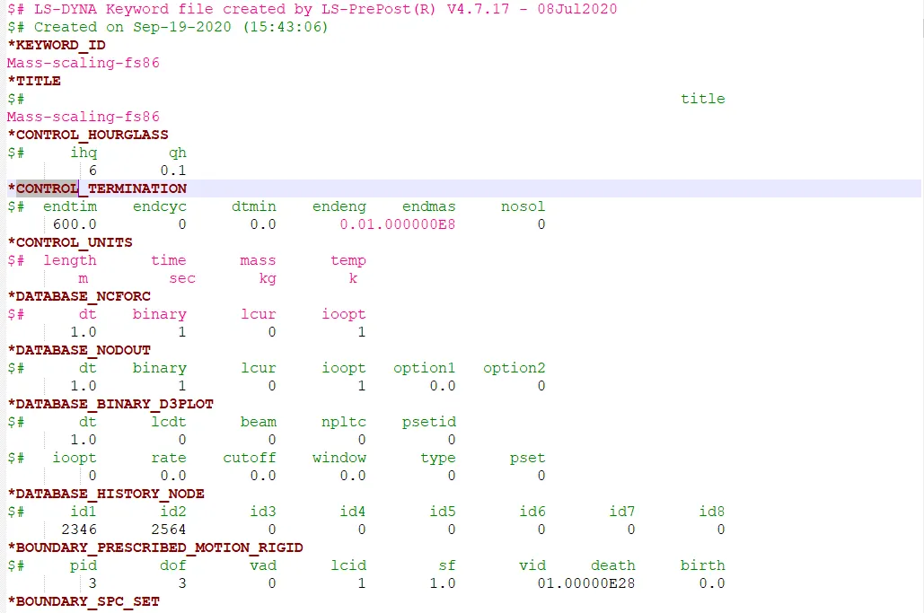
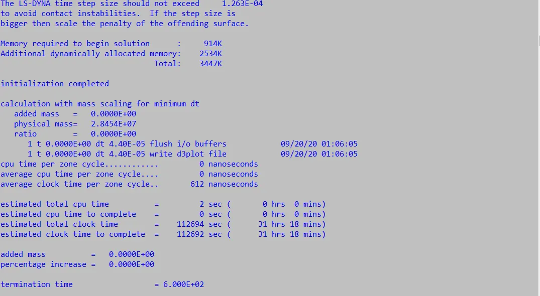
A total runtime of 23 hours was computed with a minimum time step of 4.40e-5 seconds. The very large 600 seconds end time is one of the reasons for such high run time.

Case 2:

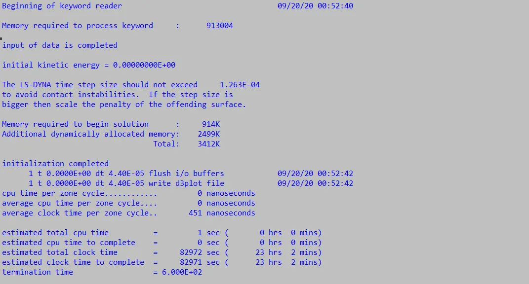
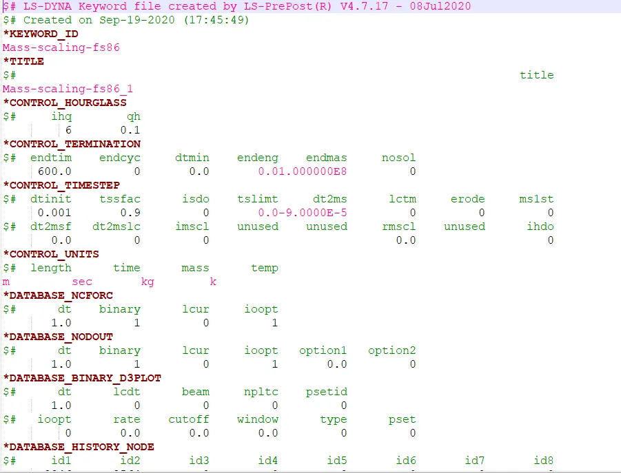
Here the control_timestep card is used with and ‘dt2ms’ figure of 3.5e-5, which is lower than the calculated minimum time-step as seen in case 1.

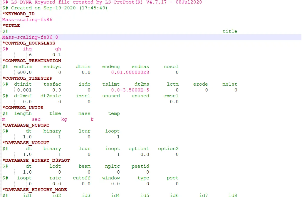
As expected by lowering the minimum time step, the calculated total runtime is increased to 31 hours.

Case 3:

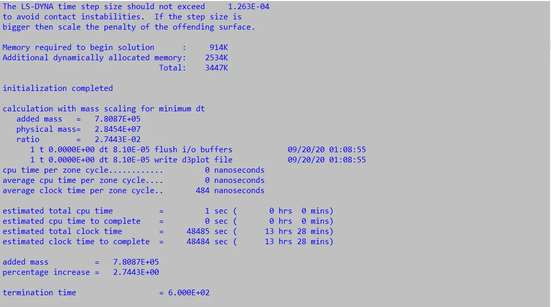
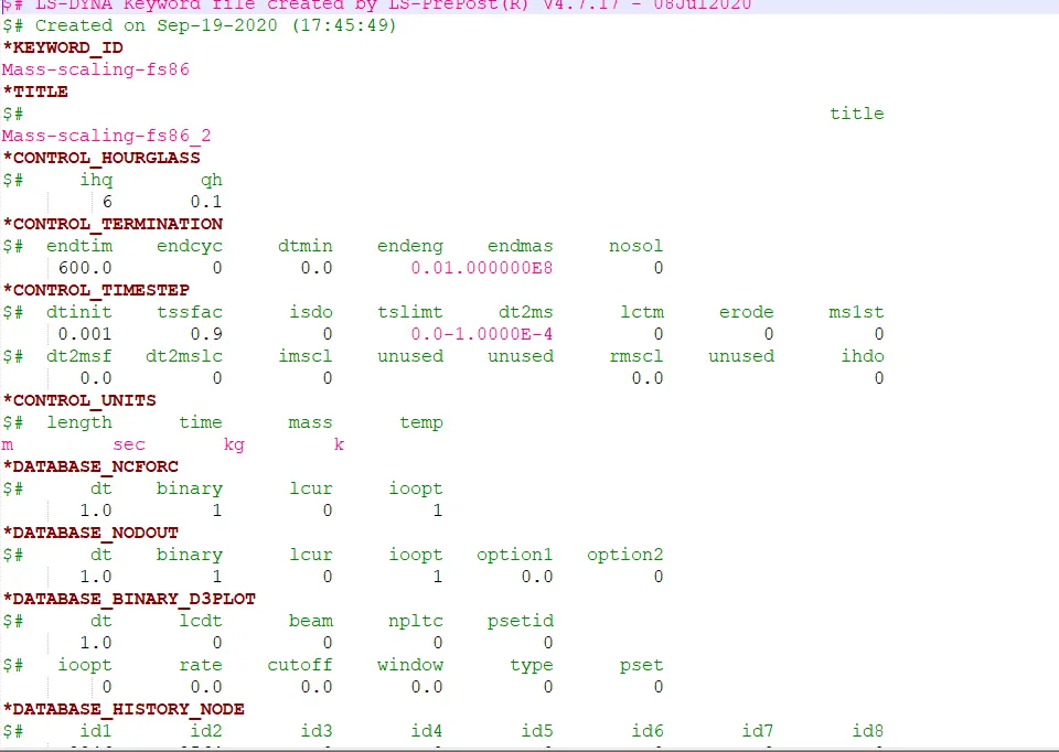
This is the 1^st iteration in mass scaling. An increase in the minimum time-step is achieved by adding mass. The ‘dt2ms’ figure was changed to 9e-5 which is a bit higher than the default 3.5e-5. This is achieved by adding 7.8e5 Kg mass to elements with lower time-step as per the relation mentioned before. This comes out to be 2.7% mass addition to the original mass.

As expected, the runtime is reduced drastically to 13 hours.

Case 4:

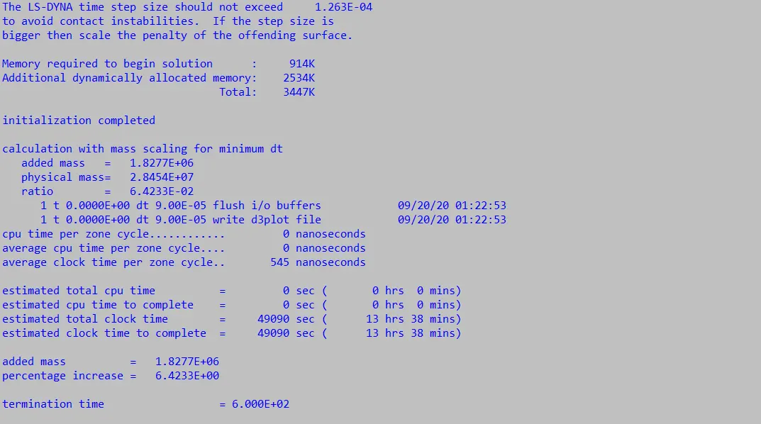
The ‘dt2ms’ figure is further increase to 1e-4 seconds. The added mass comes up to be 6.4%.

As the increase in minimum time-step is small there is no significant decrease in runtime. A small increase is observed on the contrary.

Case 5:

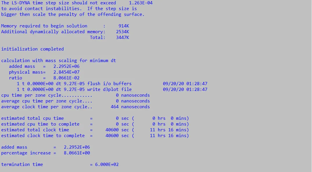
As we reach the 8% added mass limit, the increments in ‘dt2ms’ figure are reduced. In this case, the figure is kept at 1.030e-4.

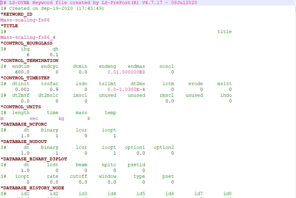
A further decrease in run time is observed – down to 11 hours from previous 13. The added mass limit of 8% is reached

Implicit analysis:

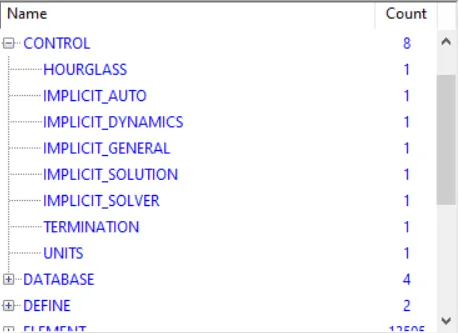
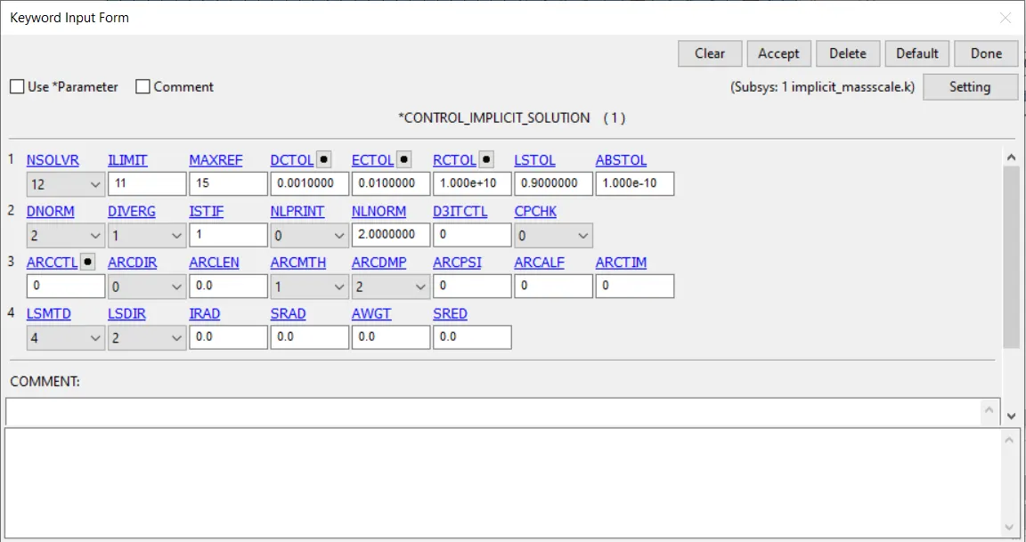
For comparison the same analysis was performed using implicit analysis method. The necessary control_implicit cards were added with default parameters for fairness.

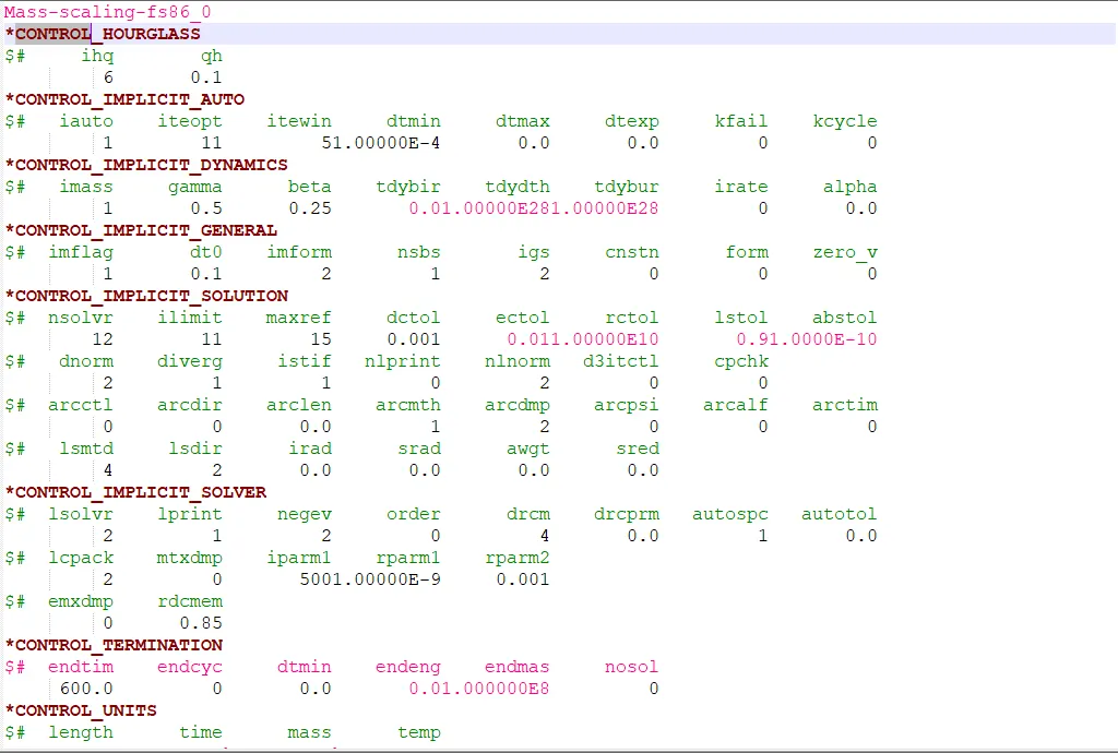
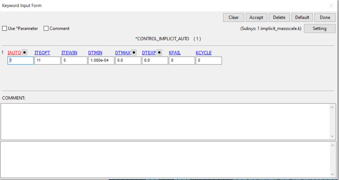
Implicit auto:

Implicit solution:

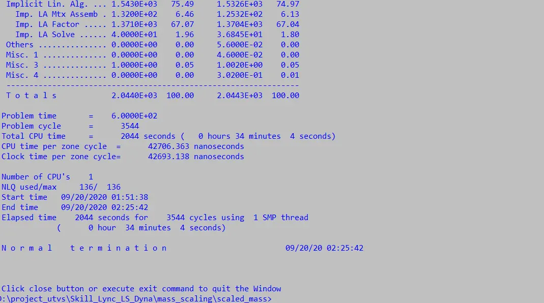
After going on with the analysis, the runtime was calculated. Implicit analysis is more useful where the simulation time is large such as the given case. As the solution needs to be converged at each time step to complete the whole analysis, larger time steps can be considered with the use of ‘dtmin’ option in the implicit auto card. This ensures faster computation without compromising accuracy.

As expected, the runtime for the implicit analysis with the same setup is significantly low at 34 minutes.

Overview of the exercise:

Sr. No.	‘dt2ms’ figure (seconds)	Analysis Run time (seconds)
1	No mass scaling	82972
2	3.5e-5	112692
3	9e-5	48484
4	1e-4	49090
5	1.025e-4	41980
6	1.03e-4	40600
7	Implicit analysis	2044

Conclusion:

1. From the comparison if different cases, it can be concluded that using mass scale can significantly bring down the analysis run time without affecting the outcomes. It is always a good practice to run the analysis without mass scaling to get an idea of the minimum time step computed by the solver and then scale it up using mass scaling if required.
2. The additional mass limit should be considered and followed strictly especially in impact, crash analysis.
3. For the given example it is clear that an implicit analysis would be the best option as it takes a fraction of the time compared to explicit cases with similar results. This also confirms the argument that explicit analysis should be used for short time dynamic analysis, whereas a longer end time analysis will always be impractical. Implicit analysis method has the advantage that the user can decide on the time-steps and hence are versatile and can be used in a number of ways.
4. Using 'tssfac' option doesn't make sense in such a case where it cannot be very effective the reason being the small margins of the time steps. With a 'tssfac' turned down to '0.7', the 'effective minimum timestep' for a 'dt2ms' figure of say 9e-5 seconds would be 0.63e-4 or 6.3e-5 which drastically changes the runtime, and hence is avoided.