Week 8 - Simulation of a backward facing step in OpenFOAM
Week 8 -
Simulation of a backward facing step in OpenFOAM
Question :
In this challenge, you are going to simulate an incompressible-laminar-viscous flow through the backward facing step geometry. You should perform a transient simulation. The solver can be chosen based on the described physics of the flow. You need to explain the entire simulation procedure (how you set up the case). You should also provide explanations to every change you make inside the reference case files obtained from OpenFOAM tutorials. You can choose the inlet velocity such that the flow is laminar.
After that, you will perform 2 case studies as described below and compare the results.
Case 1 - Simulate the flow without using any grading factor (GF = 1)
Case 2 - Simulate the flow with grading factor of 0.2. The cells should be finer near the walls (including the step wall).
You can use the following mesh parameters but you can feel free to modify these values.
Mesh specification
Number of cells along the x direction (longer dimension) = 200
Number of cells along the longer y direction = 20;
Boundary condition specification
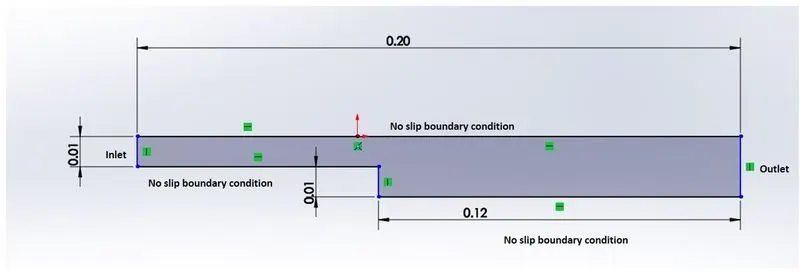
The domain specifications are provided in the following figure.
Desired output
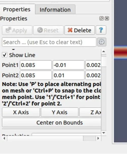
Measure the velocity profile at 0.085 m from the inlet of the geometry for both case studies and compare. You can use the plot over line tool for this.
Explain why Grading/Growth factor is essential for meshing.
Aim :
To carry out a transient simulation to simulate an incompressible-laminar-viscous flow through the backward facing step geometry.
Key Points :
- Commands using in OpenFoam and Simulation
- Creating geometry.
- Simulate the flow without using any grading factor (GF = 1)
- Simulate flow for Grading Factor 0.2
- Grading factor, Coarse and Fine mesh
Commands using in OpenFoam :-
- ls - list of all files that stored in the directories.
- cd - To change directory
- cd .. - To go back in the previous directory.
- pwd - Present working directory.
- mkdir - To create directory.
- cp - To copy
- tut - tutorials of openfoam
- app - applications
- rm - to remove files
- rm -r - to remove directories
- gedit - used to open text editors
- sol - solvers
- $FOAM_RUN - navigates to openfoam run directory
- paraFoam - opens paraview where the simulation is represented.
Steps Involved in Simulation :-
We are going to simulate our problem in OpenFOAM and solve our problem using the tutorial file present in OpenFOAM.
- Open the new terminal of OpenFoam through ubuntu.
- Type “tut” to open the tutorial directory and then type 'ls' to see what kind of file is present inside the directory.
- As it is an incompressible flow, we navigate into the incompressible directory. We use the “cd” command to navigate and change the working directory using the terminal window.
- The next step involves navigating into the icoFoam The icoFoam command solves the incompressible laminar Navier-Stokes equations. The code is inherently transient, requiring an initial condition (such as zero velocity) and boundary conditions. Therefore selecting this folder by typing “cd icoFoam” and then using the “ls” command for exploring the folder.
- Here we have two options cavity and elbow, they both are part of the icoFoam solver. Here we use the cavity folder for our required domain. But we are not going to make any changes here in the tutorial section, because OpenFOAM does not allow us to make any changes to their official tutorials.
- Here, we use the cavity utility to create our required domain. We copy this directory into the $FOAM_RUN file, which is a default file OpenFOAM creates for us. We use the “cp -r” command to recursively create a copy of the contents of the file or directory into the $FOAM_RUN folder under the file name “back_step_simulation”, for personal use. We create a copy of the files as OpenFOAM does not let us modify or make changes to its inbuilt tutorial files.
- We then navigate to the copied tutorial file in the $FOAM_RUN directory to view the contents inside the folder.
- Open back_step_simulation folder, here we can provide the specification for our block mesh in a system folder.
We can see above steps in following image
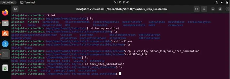
- There are 4 script file system folders and by opening blockMeshdict, we can create a domain and provide the specification for block mesh. So open this file by typing “gedit blockMeshdict”. Now make required changes in the blockMeshdict script file.
Creating a Geometry :-
The domain specifications are provided in the following figure and to create the geometry we need to edit the blockMeshdict file.
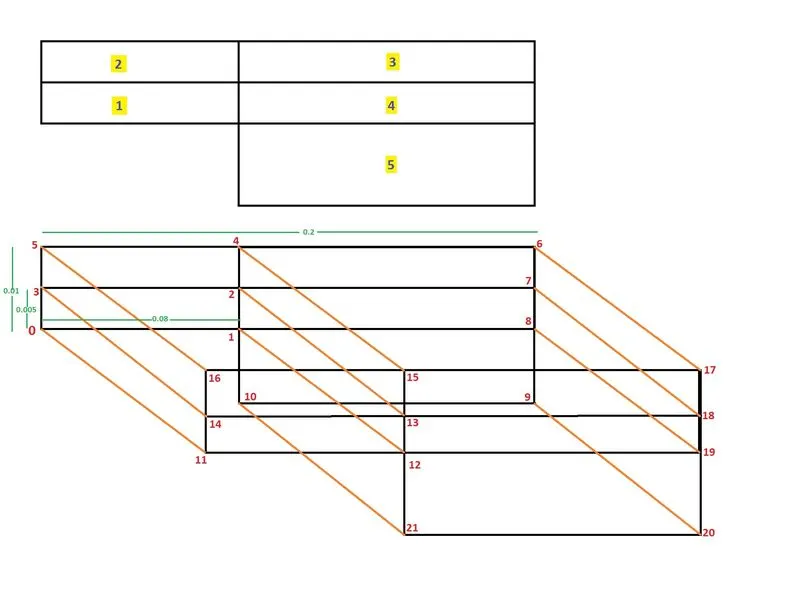
With reference to these vertices, we are going to be making certain modifications in the source codes so as to meet our specifications. They are as follows.
Case 1 - Simulate the flow without using any grading factor (GF = 1)
Case 2 - Simulate the flow with grading factor of 0.2. The cells should be finer near the walls (including the step wall).
CASE - 1 : Simulate the flow without using any grading factor (GF = 1)
Defining the Vertices :-
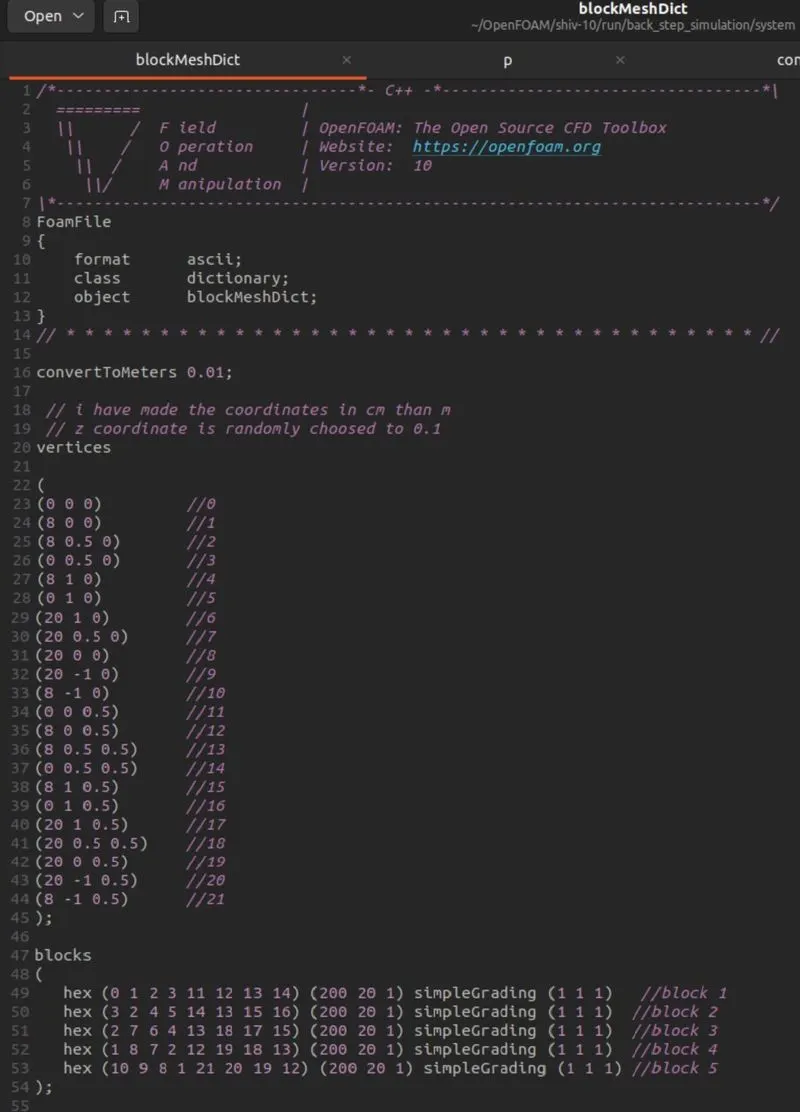
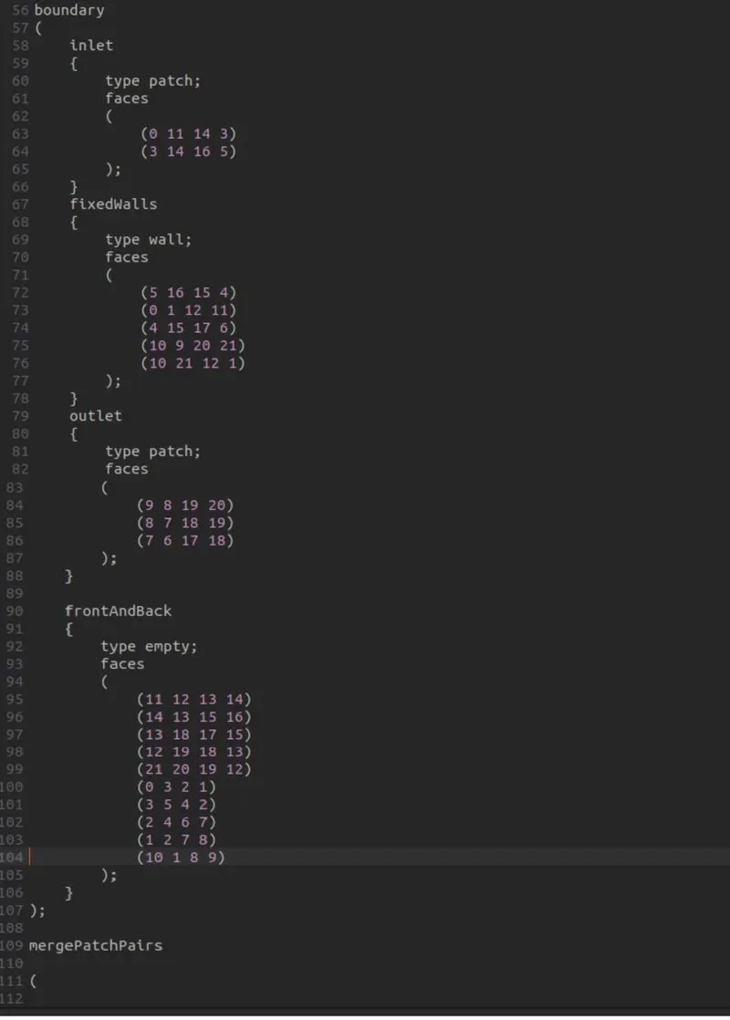
The blockMeshDict file contains the following parts,
i) The first 7 lines of the file is called the Header, which are commands and are non-executable.
ii) The next part of the file (lines 8 – 14) is referred to as the file identifier. The FoamFile line represents the software corresponding to the file is OpenFOAM. The structure of this part is referred to as a dictionary and it contains key-value pairs.
iii) The next line (line 16) is define conversation factor. It converts defined length into meters.
iv) The next part of the file are the defined vertices of the blocks, which are the respective co-ordinates which we specify in an order obeying the right hand thumb rule.
controlDict file :
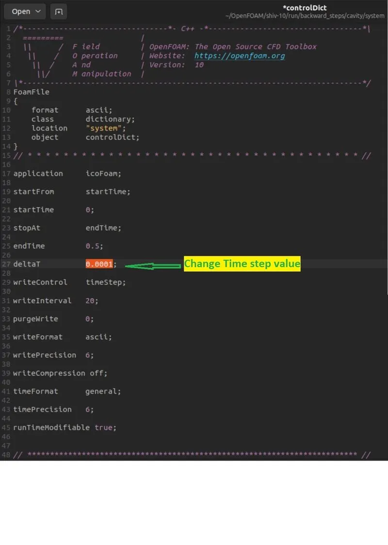
After finishing the modifications to the blockMeshDict file, we move on further to make the necessary changes to our controlDict file. In this file, we define the time interval for which our simulation is supposed to run (simulation time) and also the timestep value for the same, as shown below.
We do not make any further changes to the “fvSchemes” and “fvSolution” files in our system folder.
Initial Conditions :
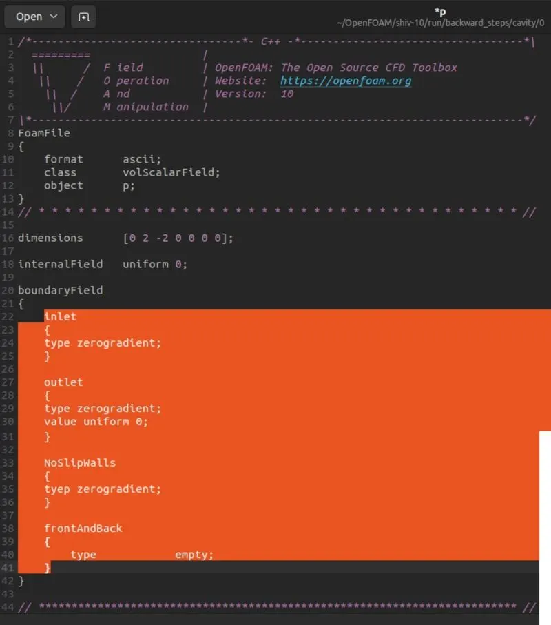
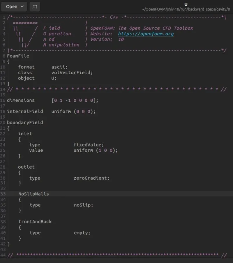
We navigate into the initial value folder (0) of the cavity test file to modify the initial values for velocity (U) and pressure (p) respectively.
Setting the initial profiles for U and p
Initial setup for pressure:
Setup for Velocity:
After completion of all the above mentioned steps, we then use the “blockMesh” command to create a mesh model of our geometry, with the number of cells along x and y – axes as previously specified above.
After creation of the meshed model, we finally use the “icoFoam” command to run the simulation for the same to obtain our final results.
After that we use “paraFoam” command to open ParaView Model.
Click apply button on left side of paraView model and select “Surface with Edges” option fron center tab “Surface”.
To view velocity profile, select “U” from “VtkBlockColors” tab left side to surface tab. Select “Surface” option fron center tab “Surface with Edges”.
Also from left bottom corner go into Properties – Fields and remove “P” as shown below and click on Apply. To play animation click on Play tab above surface tab
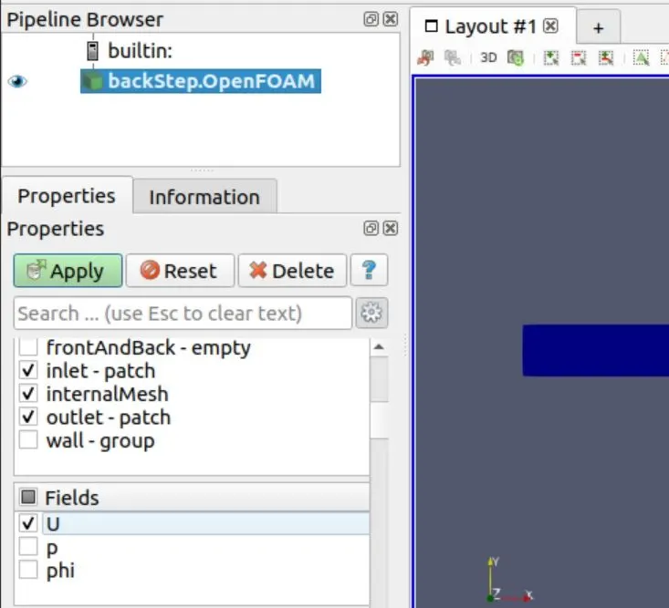
To plot graph of velocity profile select option “Plot Over Line” below “Surface” tab and also change axis from properties.
Click on Y axis and change co-ordinates of point 1 and point 2 as shown below and then click on apply
Output :-
- Mesh Generation :-
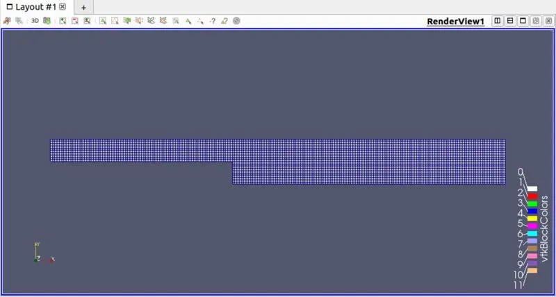
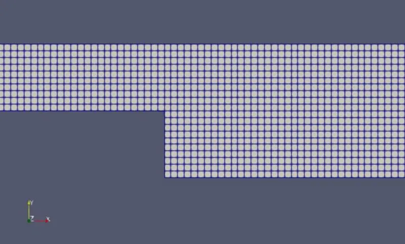
Detailed Mesh
- Velocity Distribution :-
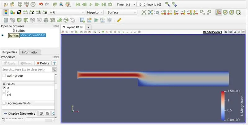
- Velocity Profile :-
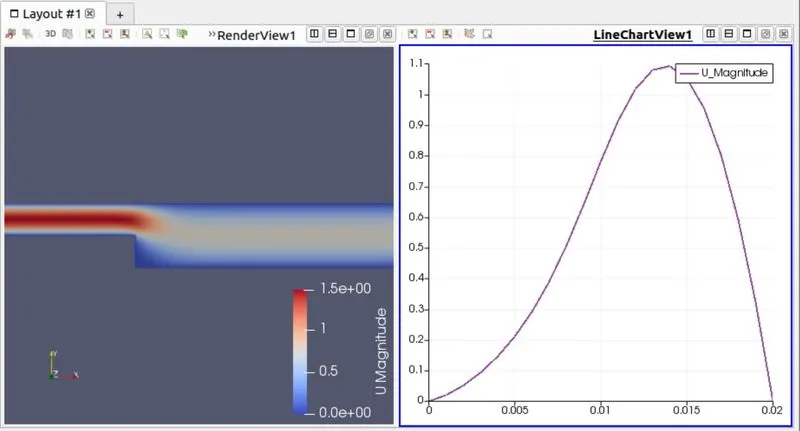
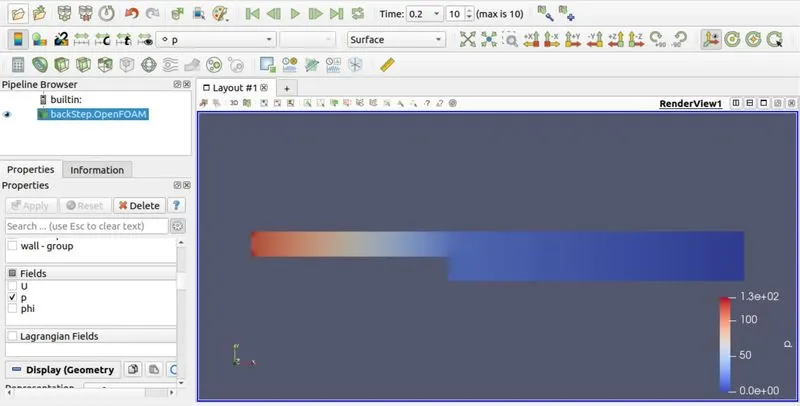
4. Pressure Distribution :-
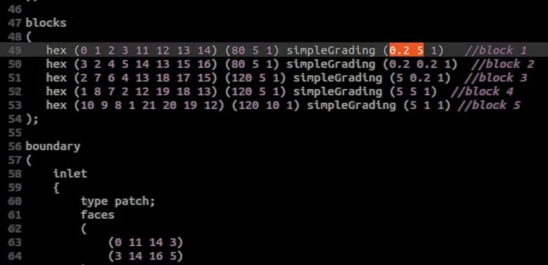
CASE - 2 : Simulate the flow with grading factor of 0.2 (GF = 0.2)
For changing grading factor to 0.2, we will make changes in blockMeshDict file only. In that file we will change grading factors for blocks only as shown below.
Why is grading / growth factor essential for meshing ?
Mesh Grading basically refers to a technique called mesh stretching, which helps us to stretch the mesh along any particular direction (x , y or z direction). This helps us in increasing the computational efficiency of the simulations.
Mesh Grade=(Size of End Cell)/(Size of Starting Cell)
The goal of meshing in CFD is to obtain the best mesh possible without sacrificing reasonable accuracy. A finer mesh at the areas where the fluid shows large changes, leads to higher accuracy. Thereby, we use a finer mesh around the walls of the geometry and also around the point where we expect our results.
Coarse and Fine Mesh :
A coarse mesh is the one where mesh elements are kept bigger such that they accommodate the geometry with less number of total mesh elements. Coarse mesh is generally what the CFD/FEA simulation is initially run with and then the mesh is refined further until we reach the point of validation where the results are no longer mesh dependent.
A refined mesh is basically a finer mesh with smaller elements. When the geometry has features like sharp angles, edges, etc. a relatively finer mesh is required to capture them.
Output :-
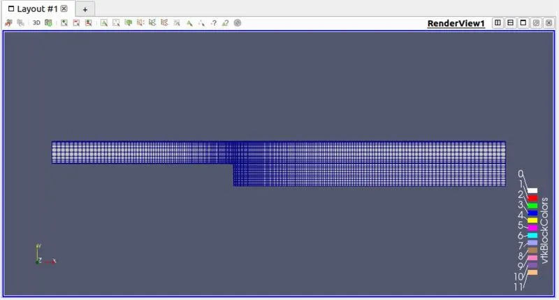
- Mesh Generation :-
Detailed Mesh
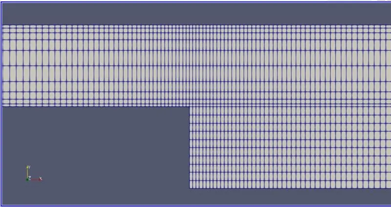
- Velocity Distribution :-
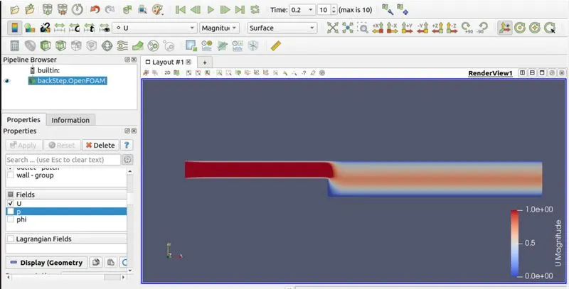
3. Velocity Profile :-
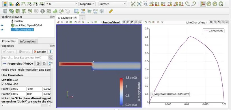
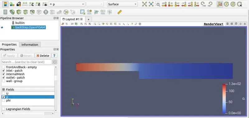
- Pressure Distribution :-
Conclusion:
- From the above case studies, we can observe that a finer mesh around the regions where large motion of the fluid occurs, leads to much accurate results when compared to that of a normal or coarse mesh region. Thereby, we can conclude that using a fine mesh around the regions or the walls where there is higher fluid interaction, leads to more accurate results wherein we can more clearly capture these changes more accurately.
- Varying the mesh quality and the grading factor will have a straight impact on the velocity and the pressure.
Reference: