Week 4.1 - Genetic Algorithm
Genetic Algorithm
Aim :
Write a code in MATLAB to optimise the stalagmite function and find the global maxima of the function.
Objective :
- Write a code in MATLAB to optimise the stalagmite function and find the global maxima of the function.
- Clearly explain the concept of genetic algorithm in your own words and also explain the syntax for ga in MATLAB in your report.
- Make sure that your code gives the same output, even if it is made to run several times.
- Plot graphs for all 3 studies and for F maximum vs no. of iterations. Title and axes labels are a must, legends could be shown if necessary.
Body of the content:
What is Genetic Algorithm?
A genetic algorithm is a method for solving both constrained and unconstrained optimization problems based on a natural selection process that mimics biological evolution. The algorithm repeatedly modifies a population of individual solutions.
GAs operate on a population of potential solutions applying the principle of survival of the fittest to produce better and better approximations to a solution. At each generation, a new set of approximations is created by the process of selecting individuals according to their level of fitness in the problem domain and breeding them together using operators borrowed from natural genetics. This process leads to the evolution of populations of individuals that are better suited to their environment than the individuals that they were created from, just as in natural adaptation.
For example, a problem with two variables, x1 and x2, may be mapped onto the chromosome structure in the following way:
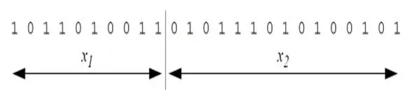
where x1 is encoded with 10 bits and x2 with 15 bits, possibly reflecting the level of accuracy or range of the individual decision variables. Examining the chromosome string in isolation yields no information about the problem we are trying to solve. It is only with the decoding of the chromosome into its phenotypic values that any meaning can be applied to the representation. However, as described below, the search process will operate on this encoding of the decision variables, rather than the decision variables themselves, except, of course, where real-valued genes are used. Having decoded the chromosome representation into the decision variable domain, it is possible to assess the performance, or fitness, of individual members of a population. This is done through an objective function that characterises an individual’s performance in the problem domain.
In the natural world, this would be an individual’s ability to survive in its present environment. Thus, the objective function establishes the basis for selection of pairs of individuals that will be mated together during reproduction.
During the reproduction phase, each individual is assigned a fitness value derived from its raw performance measure given by the objective function. This value is used in the selection to bias towards more fit individuals. Highly fit individuals, relative to the whole population, have a high probability of being selected for mating whereas less fit individuals have a correspondingly low probability of being selected.
Once the individuals have been assigned a fitness value, they can be chosen from the population, with a probability according to their relative fitness, and recombined to produce the next generation. Genetic operators manipulate the characters (genes) of the chromosomes directly, using the assumption that certain individual’s gene codes, on average, produce fitter individuals. The recombination operator is used to exchange genetic information between pairs, or larger groups,
of individuals. The simplest recombination operator is that of single-point crossover.
Consider the two parent binary strings:
P1 = 1 0 0 1 0 1 1 0, and
P2 = 1 0 1 1 1 0 0 0.
If an integer position, i, is selected uniformly at random between 1 and the string length, l, minus one [1, l-1], and the genetic information exchanged between the individuals about this point, then two new offspring strings are produced. The two offspring below are produced when the crossover point i = 5 is selected,
O1 = 1 0 0 1 0 0 0 0, and
O2 = 1 0 1 1 1 1 1 0.
This crossover operation is not necessarily performed on all strings in the population. Instead, it is applied with a probability Px when the pairs are chosen for breeding. A further genetic operator, called mutation, is then applied to the new chromosomes, again with a set probability, Pm. Mutation causes the individual genetic representation to be changed according to some probabilistic rule. In the binary string representation, mutation will cause a single bit to change its state, 0 ⇒ 1 or 1 ⇒ 0. So, for example, mutating the fourth bit of O1 leads to the new string,
O1m = 1 0 0 0 0 0 0 0.
Mutation is generally considered to be a background operator that ensures that the probability of searching a particular subspace of the problem space is never zero.
This has the effect of tending to inhibit the possibility of converging to a local optimum, rather than the global optimum. After recombination and mutation, the individual strings are then, if necessary, decoded, the objective function evaluated, a fitness value assigned to each individual and individuals selected for mating according to their fitness, and so the process continues through subsequent generations. In this way, the average performance of individuals in a population is expected to increase, as good individuals are preserved and bred with one another and the less fit individuals die out. The GA is terminated when some criteria are satisfied, e.g. a certain number of generations, a mean deviation in the population, or when a particular point in the search space is encountered.
GAs versus Traditional Methods
From the above discussion, it can be seen that the GA differs substantially from more traditional search and optimization methods.
The four most significant differences are:
- GAs search a population of points in parallel, not a single point.
- GAs do not require derivative information or other auxiliary knowledge; only the objective function and corresponding fitness levels influence the directions of search.
- GAs use probabilistic transition rules, not deterministic ones.
- GAs work on an encoding of the parameter set rather than the parameter set itself (except in where real-valued individuals are used).
It is important to note that the GA provides a number of potential solutions to a given problem and the choice of final solution is left to the user. In cases where a particular problem does not have one individual solution, for example a family of Pareto-optimal solutions, as is the case in multi objective optimization and scheduling problems, then the GA is potentially useful for identifying these alternative solutions simultaneously.
The simple genetic algorithm (SGA) is described by Goldberg and is used here to illustrate the basic components of the GA. A pseudo-code outline of the SGA is shown in Fig. 1. The population at time t is represented by the time-dependent
variable P, with the initial population of random estimates being P(0). Using this outline of a GA, the remainder of this Section describes the major elements of the GA.
procedure GA
begin
t = 0;
initialize P(t);
evaluate P(t);
while not finished do
begin
t = t + 1;
select P(t) from P(t-1);
reproduce pairs in P(t);
evaluate P(t);
end
end.
Figure 1: A Simple Genetic Algorithm
Basic Structure
The basic structure of a GA is as follows −
We start with an initial population (which may be generated at random or seeded by other heuristics), select parents from this population for mating. Apply crossover and mutation operators on the parents to generate new off-springs. And finally these off-springs replace the existing individuals in the population and the process repeats. In this way genetic algorithms actually try to mimic the human evolution to some extent.
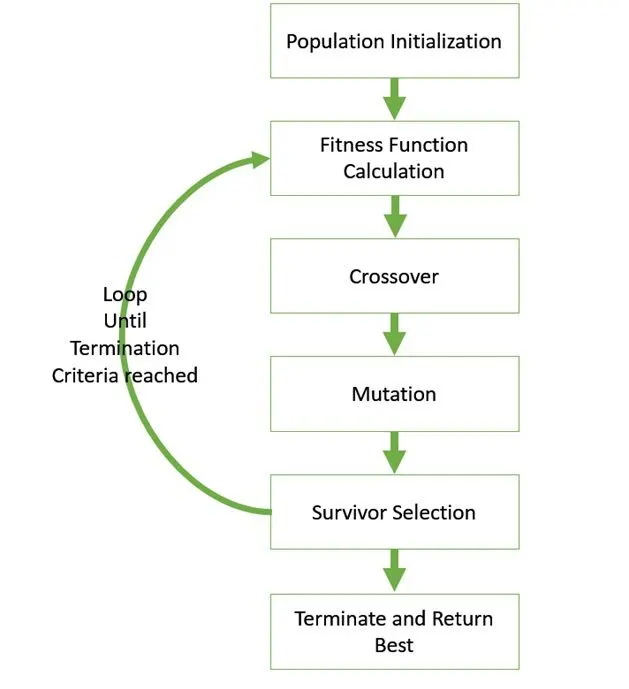
Stopping Criteria:
GA stops when it reaches the maximum number of generations; by default, this number is 100 times the number of variables.
Fitness Limit — The algorithm stops when the value of the fitness function for the best point in the current population is less than or equal to Fitness Limit .
Syntax Used for Genetic Algorithm
X = ga(fun, nvars) Find local unconstrained minimum, x, to the objective function, fun.
nvars is the dimension (number of design variables) of fun.
X = ga(fun, nvars,A,b) Find local minimum x to fun, subject to linear inequalities A*x ≤ b.
ga evaluates the matrix product A*x as if X is transposed (A*X’)
X = ga(fun, nvars,A,b,Aeq,beq) Find local minimum x to fun, subject to linear inequalities Aeq*x= beq and A*X ≤ b.
Set A=[] and b=[] if no linear inequalities exist).
ga evaluates the matrix product Aeq*x as if X is transposed (Aeq*X’)
X = ga(fun, nvars,A,b,Aeq,beq,lb,ub) defines lower and upper bound on design variables ,x, so that solution is found in the range lb ≤ X ≤ ub
X = ga(fun, nvars,A,b,Aeq,beq,lb,ub,nonlcon) subjects the minimization to the constrain defined in nonlcon. The function nonlcon accepts X and returns vector C and Ceq.
Representing the nonlinear inequalities and equalities respectively .ga minimize the function such that C(X) ≤ 0 and Ceq(X) = 0
(set lb = [] and ub = [] is no bound exists.)
X = ga(fun, nvars,A,b,Aeq,beq,lb,ub,nonlcon,options) minimizes the default optimizations parameters replaced by values in options.
(set nonlcon = [] if no linear constrains exists.)
Create options using optimoptions
X = ga(fun, nvars,A,b,Aeq,beq,lb,ub,nonlcon,Intcon) requires that the variables listed in Intcon take integer value
Governing Equation:
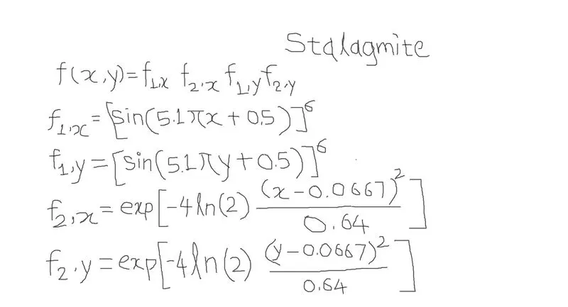
Program
Programming Language: MATLAB
# First create program for stalagmite function by dividing governing equation into 4 terms.
Stalagmite function
%define stalagmite function

function[f] = stalagmite(input_vector)
x = input_vector(1);
y = input_vector(2);

t1 =(sin((5.1*pi*x)+0.5)).^6;
t2 =(sin((5.1*pi*y)+0.5)).^6;
t3 =exp((-4)*log(2)*((x-0.0667).^2)/0.64);
t4 =exp((-4)*log(2)*((y-0.0667).^2)/0.64);

% -ve sign to find out maxima

f =-(t1*t2*t3*t4);
end
# Now in main code define 2 inputs X and Y. These both are one dimensional equally spaced array containing 100 elements.
# Use meshgrid command to create array of X and Y values.
# Now we use for loop to input values of 2D array in stalagmite function. Every time code is executed different values for stalagmite function are obtained. This problem can be overcome by introducing another loop into code.
# Using new inputs and ga function code for generic algorithm is created.
To find global maxima of function we consider 3 cases.
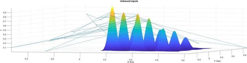
Case 1: Unbounded Inputs
In this case evaluate all possible global maxima for all iteration without considering boundaries of X and Y.
# Plot 2 graphs in one fig. using subplot command.
# tic and toc commands are used to evaluate time taken for optimizing function and value stored into case1_time
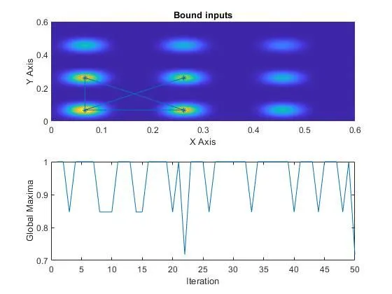
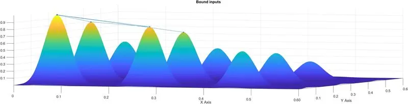
Case 2: Bounded Inputs
In this case put upper and lower bound on ga function and evaluate all possible global maxima for all iteration considering boundaries of X and Y.
Case 3: Increase ga Iterations
In this case we increase ga iteration, by doing this we can achieve optimal solution because in GA after successive iteration the population evolves towards an optimal solution.
Main Code
clear all
close all
clc

% Define search space
x = linspace(0,0.6,150);
y = linspace(0,0.6,150);

limit = 50;

% Creating 2 Dimensional mesh
[xx yy] = meshgrid(x, y);

% Evaluating the stalagmite function

for i = 1:length(xx)
    for j = 1:length(yy)
        input_vector(1) = xx(i,j);
        input_vector(2) = yy(i,j);
        f(i,j) = stalagmite(input_vector);
    end
end

% Case 1 %
% Statistical Behaviour with unbound inputs
tic
for i = 1:limit
[inputs, f_opt1(i)] = ga(@stalagmite, 2);

x_opt1(i) = inputs(1);
y_opt1(i) = inputs(2);
end
case1_time = toc
F = -f;
F_opt1 = -f_opt1;

figure(1)
subplot(2,1,1)
hold on
grid on
title('Unbound inputs')
surfc(xx, yy, F)
shading interp
plot3(x_opt1,y_opt1,F_opt1,'marker','X','markersize',5)
xlabel('X Axis')
ylabel('Y Axis')
zlabel('f')

subplot(2,1,2)
plot(F_opt1)
xlabel('Iteration')
ylabel('Global Maxima')

% Case 2 %
% Statistical Behaviour with bound inputs
tic
for i = 1:limit
[inputs, f_opt2(i)] = ga(@stalagmite,2,[],[],[],[],[0;0],[0.6;0.6]);

x_opt2(i) = inputs(1);
y_opt2(i) = inputs(2);
end
case2_time = toc
F_opt2 = -f_opt2;

figure(2)
subplot(2,1,1)
title('Bound inputs')
hold on
grid on
surfc(xx, yy, F)
shading interp
plot3(x_opt2,y_opt2,F_opt2,'marker','*','markersize',5)
xlabel('X Axis')
ylabel('Y Axis')

subplot(2,1,2)
plot(F_opt2)

xlabel('Iteration')
ylabel('Global Maxima')


% Case 3 %
% Increase Iterations

options = optimoptions('ga');
options = optimoptions(options, 'PopulationSize', 200);
tic
for i = 1:limit
[inputs, f_opt3(i)] = ga(@stalagmite,2,[],[],[],[],[0;0],[0.6;0.6],[],[],options);

x_opt3(i) = inputs(1);
y_opt3(i) = inputs(2);
end
case3_time = toc
F_opt3 = -f_opt3;

figure(3)
subplot(2,1,1)
title('Bound inputs with Increased population Size')
hold on
grid on
surfc(xx, yy, F)
shading interp
plot3(x_opt3,y_opt3,F_opt3,'marker','O','markersize',5)
xlabel('X Axis')
ylabel('Y Axis')

subplot(2,1,2)
plot(F_opt3)

xlabel('Iteration')
ylabel('Global Maxima')
Output Case 1: Unbound Inputs
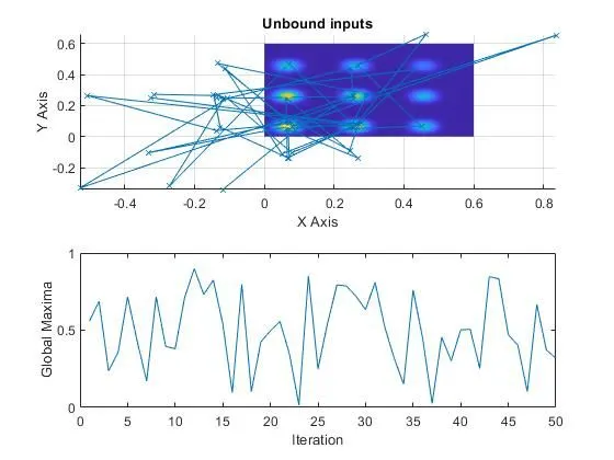
Output Case 2: Bound Inputs
Output Case 3: Increase Iteration
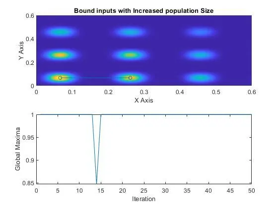
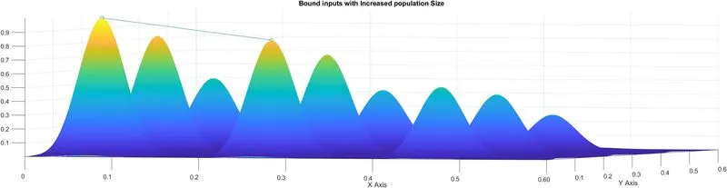
From output fig 3, the maxima of the function is said to be much more accurate and closer to true value. In case 3 it is more precise since variation between result is very less. Compared to first 2 cases , there is very little to no fluctuation.
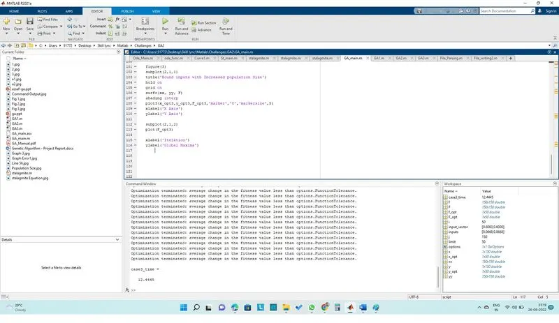
Output: Command Window
Errors
Error 1:
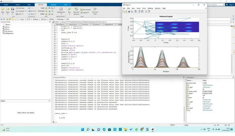
Error: Mistake in plot command of 2nd graph
Error 2
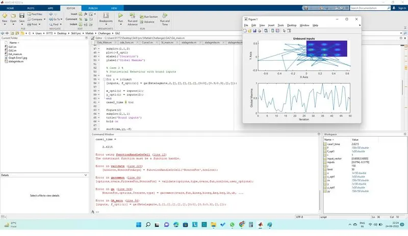
Error: Mistake in defining ga syntax
[inputs, f_opt2(i)] = ga(@stalagmite,2,[],[],[],[],[],[0;0],[0.6;0.6]);
Corrected as: Removed extra [ ] from syntax
[inputs, f_opt2(i)] = ga(@stalagmite,2,[],[],[],[],[0;0],[0.6;0.6]);
Error 3
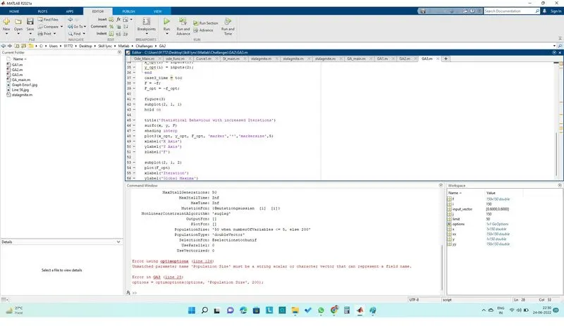
Error: Mistake in defining optimoptions syntax
options = optimoptions(options, 'Population Size', 200);
Corrected as: Remove space from PopulationSize
options = optimoptions(options, 'PopulationSize', 200);
Result
Case 1: Unbound Inputs time taken: 2.8363 Sec
Case 2: Bound Inputs time taken: 3.4973 Sec.
Case 3: Increase Iterations time taken: 8.1743 Sec.
Conclusion
Genetic Algorithm GA used as model to salve stalagmite function in order to determine global maxima.
By increasing number of iterations, increasing population size and by setting constrains in upper and lower bound the result for global maxima become optimized.
References:
- https://learnwithpanda.com/2020/07/22/genetic-algorithm-general-concept-matlab-code-and-example
- https://www.tutorialspoint.com/genetic_algorithms/genetic_algorithms_fundamentals.htm
- https://www.cs.drexel.edu/~spiros/teaching/CS675/slides/ga.ppt
- https://towardsdatascience.com/introduction-to-genetic-algorithms
- https://www.powershow.com/view4/67b44b-ZTZkM/Introduction_to_Genetic_Algorithms
- https://in.mathworks.com/help/gads/what-is-the-genetic-algorithm.html