Week 3 - Solving second order ODEs

ODE Pendulum

Aim : Write a program in Matlab\Octave that will simulate the pendulum motion

Objective : write a program that solves the following ODE. This ODE represents the equation of motion of a simple pendulum with damping.

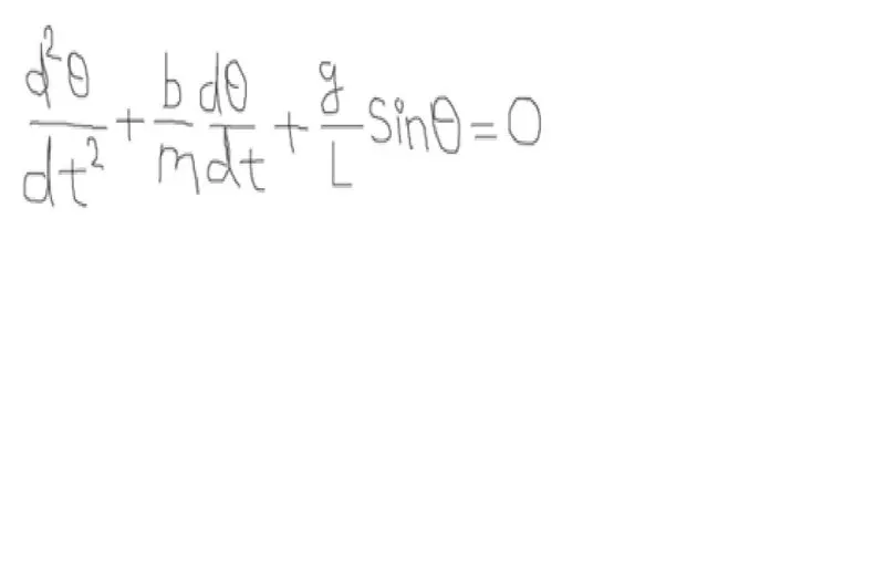
In the above equation,

g = gravity in m/s2,

L = length of the pendulum in m,

m = mass of the ball in kg,

b=damping coefficient.

Write a program in Matlab\Octave that will simulate the pendulum motion, just like the one shown in the start of this challenge.

use,

L=1 metre,

m=1 kg,

b=0.05.

g=9.81 m/s2.

Simulate the motion between 0-20 sec, for angular displacement=0, angular velocity=3 rad/sec at time t=0.

Body of the content:

Programming Language: MATLAB

ODE_main

clear all
close all
clc

l = 1;
m = 1;
b = 0.05;
g = 9.81;


% initial condition - Initial Displacement, Initial velocity
theta_0 = [0;3];

% time points
t_span = linspace(0,20,200);

% solve ODE
[t,result] = ode45(@(t,theta) ode_func(t, theta, b,g,l,m),t_span, theta_0);


%Plot graph
plot(t,result(:,1))
hold on
plot(t,result(:,2))
ylabel('Plot')
xlabel('Time')



title('Motion of Simple Pendulum');

grid on
displacement = result(:,1);
velocity = result(:,2);



ct = 1; 
% count command for the iterations 
for i = 1 : length(displacement)

    
    %Fixed co-ordinates of one end of the simple pendulum

    x0 = 0;
    y0 = 0;

    

    %Moving co-ordinates of the bob
    x1 = 1*sin(displacement(i));
    y1 = -1*cos(displacement(i));

    

    figure(2)

    % Plotting of the bob motion
    plot([-1 1],[0 0],'linewidth',4,'color','b');
    hold on;

    axis([-3 3 -3 3]);  
    
    % axis plotting

    plot([x0 x1],[y0 y1],'linewidth',3,'color','y');

    plot(x1, y1,'-O','markersize',25,'markerfacecolor','r');

    pause(0.03)

   

    M(ct) = getframe(gcf);
    ct= ct+1;
    
hold off
end



% To create animation of the simple pendulum

movie(M);
videofile = VideoWriter('Pendulum.avi','Uncompressed AVI');
open(videofile)
writeVideo(videofile,M)
close(videofile)

ode_func

function [dtheta_dt] = ode_func(t,theta,b,g,l,m)

theta1 = theta(1);
theta2 = theta(2);
% First ODE
dtheta1_dt = theta2;
% Second ODE
dtheta2_dt = -(b/m)*theta2 - (g/l)*sin(theta1);
dtheta_dt = [dtheta1_dt; dtheta2_dt];
end

Program explanation:

clear all

close all

clc

l = 1;

m = 1;

b = 0.05;

g = 9.81;

% initial condition- Initial Displacement, Initial velocity

theta_0 = [0;3];

% time points

t_span = linspace(0,20,200);

% solve ODE

[t,result] = ode45(@(t,theta) ode_func(t, theta, b,g,l,m),t_span, theta_0);

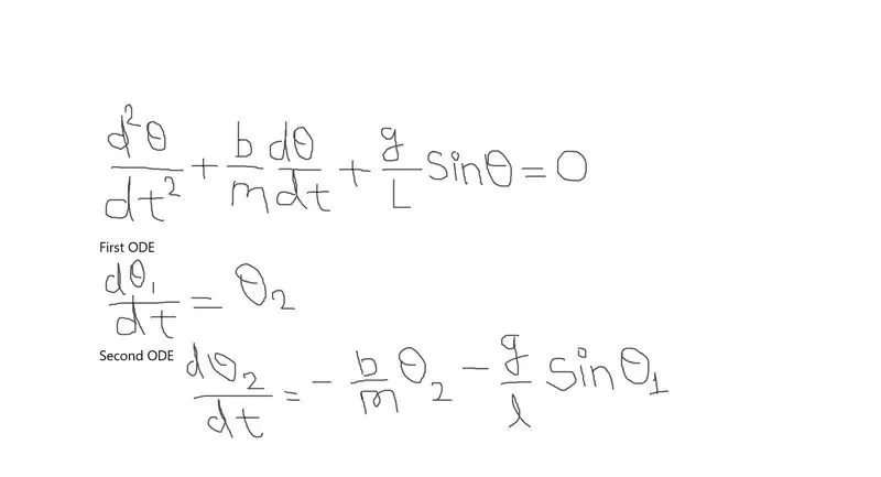
ODE Function

function [dtheta_dt] = ode_func(t,theta,b,g,l,m)

theta1 = theta(1);

theta2 = theta(2);

% First ODE

dtheta1_dt = theta2;

% Second ODE

dtheta2_dt = -(b/m)*theta2 - (g/l)*sin(theta1);

dtheta_dt = [dtheta1_dt; dtheta2_dt];

end

Again continue to Main Program

%Plot graph

plot(t,result(:,1))

hold on

plot(t,result(:,2))

ylabel('Plot')

xlabel('Time')

title('Motion of Simple Pendulum');

grid on

displacement = result(:,1);

velocity = result(:,2);

ct = 1;

% count command for the iterations

for i = 1 : length(displacement)

%Fixed co-ordinates of one end of the simple pendulum

x0 = 0;

y0 = 0;

%Moving co-ordinates of the bob

x1 = 1*sin(displacement(i));

y1 = -1*cos(displacement(i));

figure(2)

% Plotting of the bob motion

plot([-1 1],[0 0],'linewidth',4,'color','b');

hold on;

axis([-3 3 -3 3]);

% axis plotting

plot([x0 x1],[y0 y1],'linewidth',3,'color','y');

plot(x1, y1,'-O','markersize',25,'markerfacecolor','r');

pause(0.03)

M(ct) = getframe(gcf);

ct= ct+1;

hold off

end

% To create animation of the simple pendulum

movie(M);

videofile = VideoWriter('Pendulum.avi','Uncompressed AVI');

open(videofile)

writeVideo(videofile,M)

close(videofile)

Output Screenshot & Video Link:

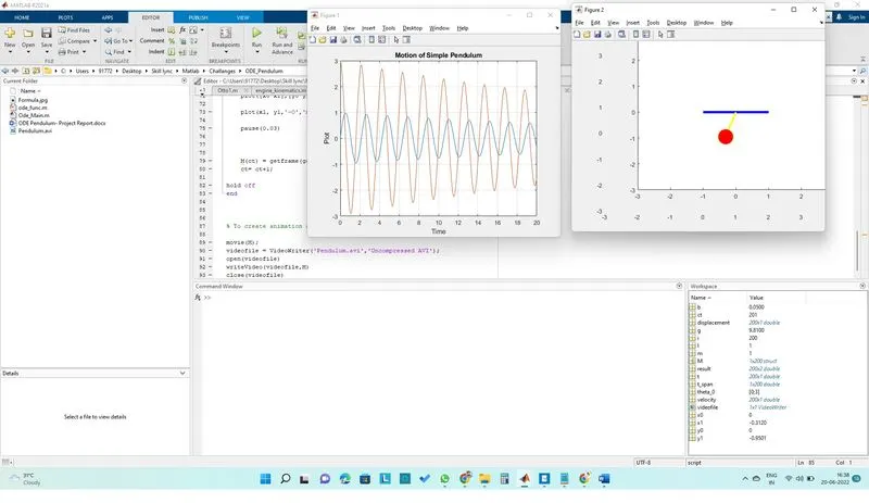
Video Link: https://youtu.be/0GCc2FG616Q

Errors:

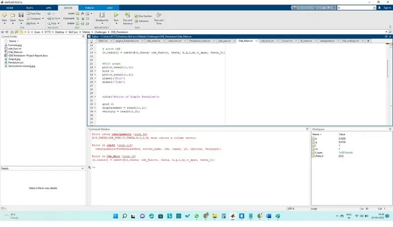
Semicolon ; is missed in function

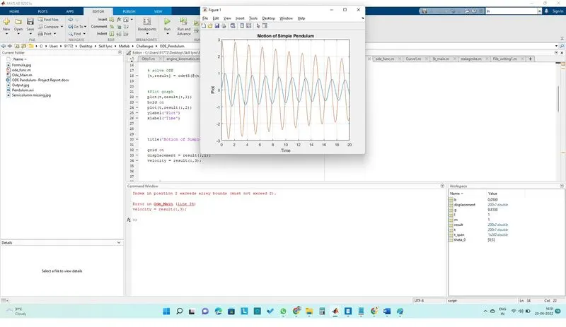
Put velocity 3 instead of 2

Corrected as follows

velocity = result(:,2);

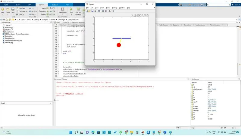
Couldn’t save video file of animation because put “M” capital in

Movie(M);

Corrected as:

movie(M);