Week - 8 Mass Scaling

REPORT - 9 ( MASS SCALING)

AIM

To reduce the run time of the model and to increase the stability of the model by mass scaling. Also, additionally, trial and error are done for the model by adding the mass to the model and once the objective is reached a histogram is plotted to compare the run time with mass scaling trials. Also, the same model is run by using implicit solver and explicit solver by making necessary changes to compare the run time between the explicit and implicit solver.

PROCEDURE FOR EXPLICIT ANALYSIS

• The file is initially opened in the LS-prepost.

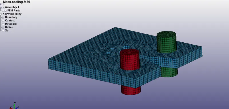
Fig, represents the mass-scaling model

• After, go to the keyword manager → control card → Timestep and change the DT2MS value to achieve the mass percentage of the model to 8 percentage.
• The trial and error method is used to find the exact value of DT2MS that is used to find the optimum percentage of mass (8%).

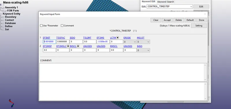
Fig, represents the change of value DT2MS(-3.5e^-5) in the *control time step

• The tssfac is kept default value to 0.9 and the simulation is solved by using LS-RUN.

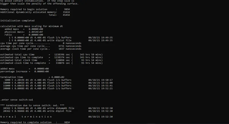
Fig, represents the percentage increase of mass for the DT2MS (-3.5e^-5)

• similarly, the values of DT2MS is changed until we achieve the percentage increase of mass to 8%.

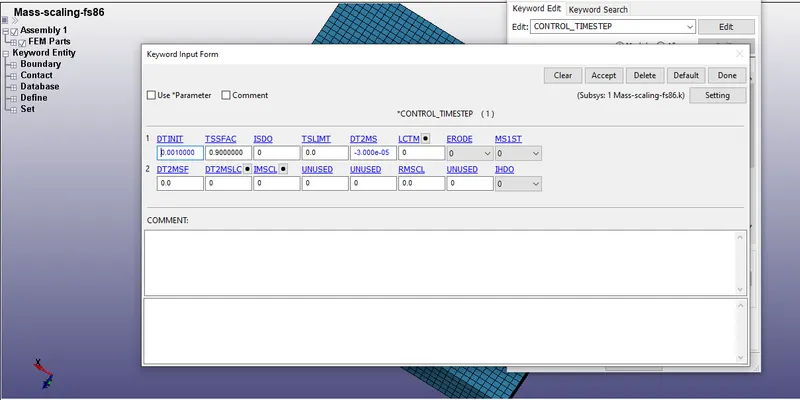
Fig, represents the change of value DT2MS(-3.0e^-5) in the *control time step

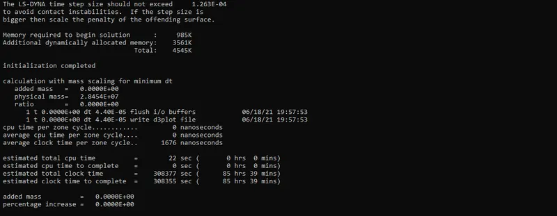
Fig, represents the percentage increase of mass for the DT2MS (-3.0e^-5)

• The same procedure is repeated by changing the other values of DT2MS.

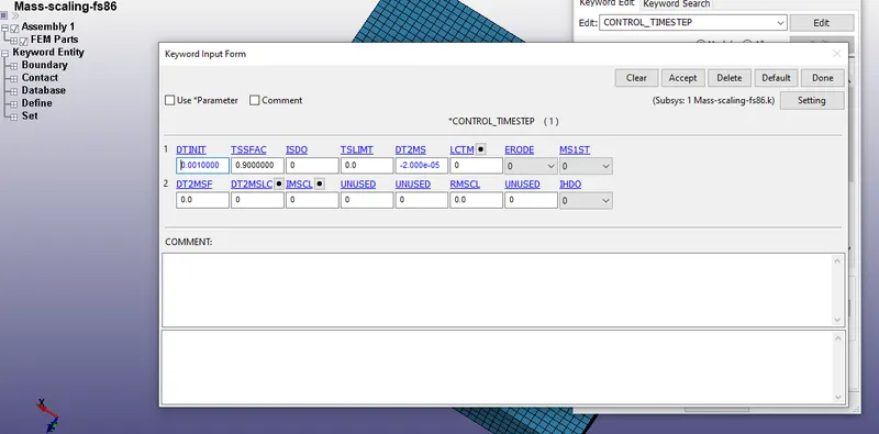
Fig, represents the change of value DT2MS(-2.0e^-5) in the *control time step

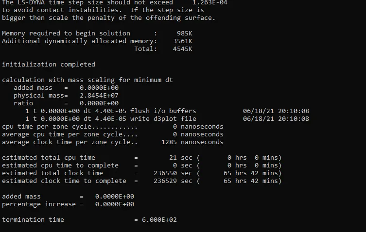
Fig, represents the percentage increase of mass for the DT2MS (-2.0e^-5)

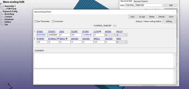
Fig, represents the change of value DT2MS(-0.50e^-5) in the *control time step

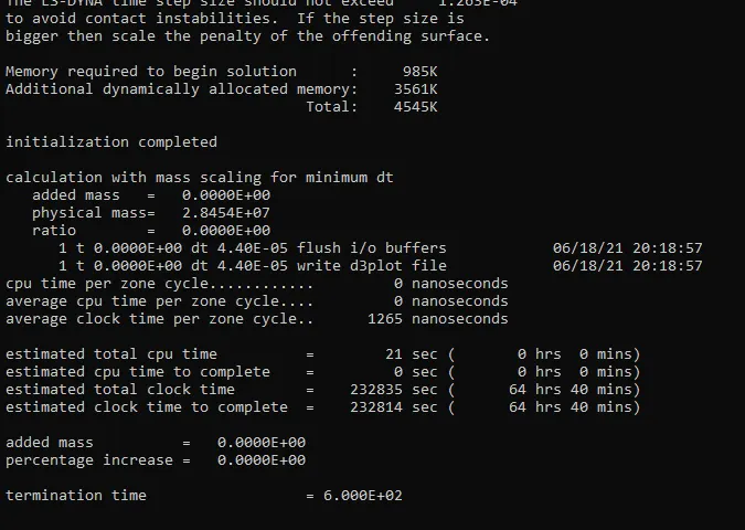
Fig, represents the percentage increase of mass for the DT2MS (-0.50e^-5)

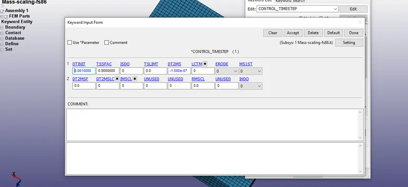
Fig, represents the change of value DT2MS(-0.1e^-5) in the *control time step

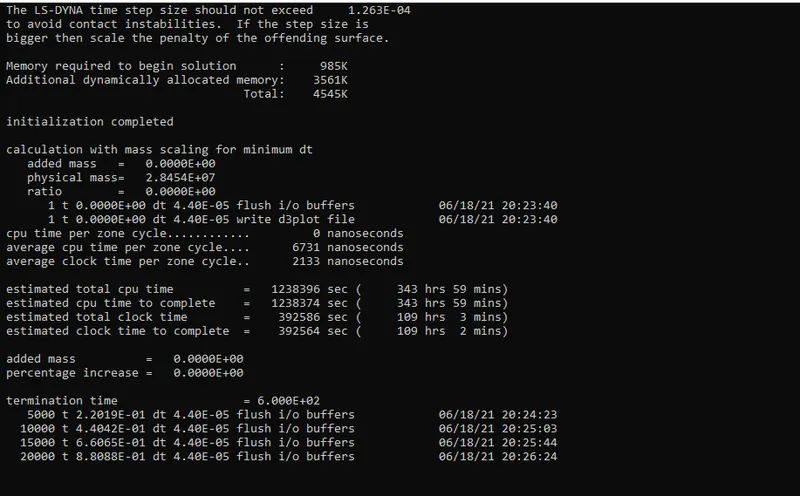
Fig, represents the percentage increase of mass for the DT2MS (-0.10e^-5)

• As we , that there was no percentage increase of mass when the values of

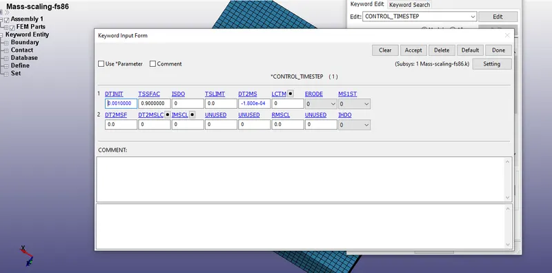
Fig, represents the change of value DT2MS(-1.8e^-4) in the *control time step

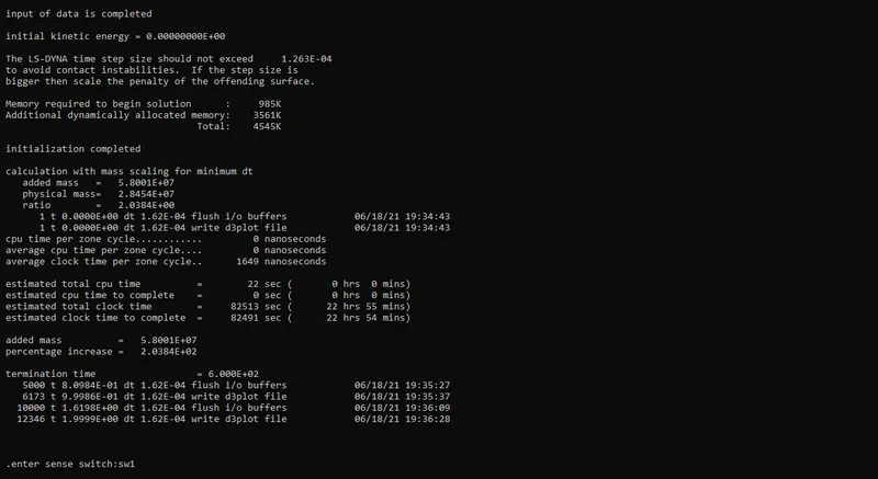
Fig, represents the percentage increase of mass (200%), for the DT2MS (-1.8e^-4)

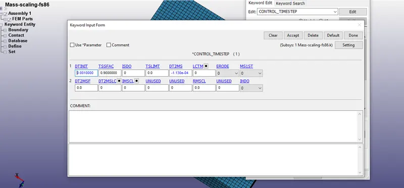
Fig, represents the change of value DT2MS(-1.13e^-4) in the *control time step

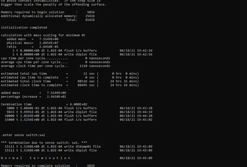
Fig, represents the percentage increase of mass (20), for the DT2MS (-1.13e^-4)

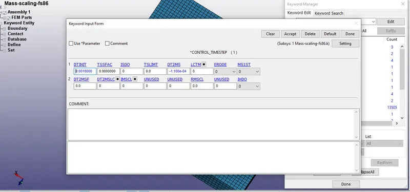
Fig, represents the change of value DT2MS(-1.10e^-4) in the *control time step

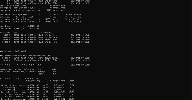
Fig, represents the percentage increase of mass (20), for the DT2MS (-1.10e^-4)

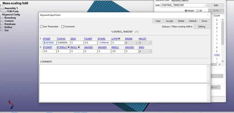
Fig, represents the change of value DT2MS(-1.5e^-4) in the *control time step

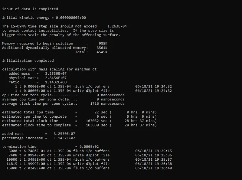
Fig, represents the percentage increase of mass, for the DT2MS (-1.5e^-4)

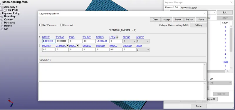
Fig, represents the change of value DT2MS(-1.03e^-4) in the *control time step

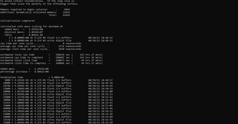
Fig, represents the increase in the percentage of mass 8% achieved for DT2MS(-1.03E^-4)

• Thus, by varying the values of DT2MS, the increase of mass 8% is achieved finally by keeping the constant value of TSSFAC to 0.9.

PROCEDURE FOR IMPLICIT ANALYSIS

• The model for mass scaling is imported for simulating the implicit analysis.
• After, go to the keyword manager → control card → Timestep→implicit general →implicit auto
• In order to do the implicit analysis, we need to activate IMFLAG1 which is present on the implicit general

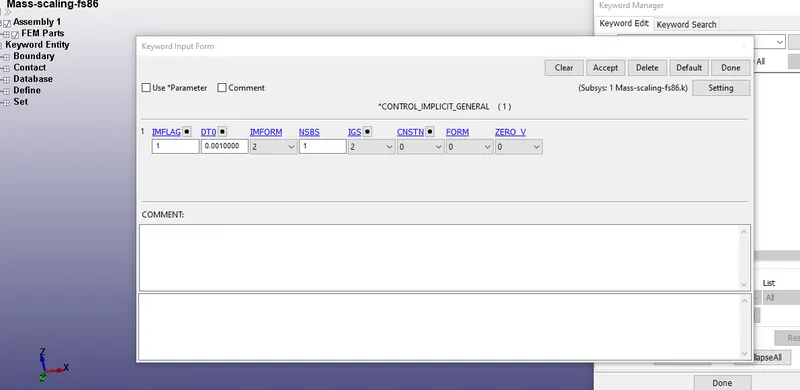
Fig, represents the IMFLAG1 for activating the implicit analysis in the control implicit card.

• In this control implicit card, a DT value of 0.001 is assigned.
• An implicit auto card is created for creating the ITEOPT (11 iterations), ITEWIN 5, this is done for optimizing the no of iterations within a range.

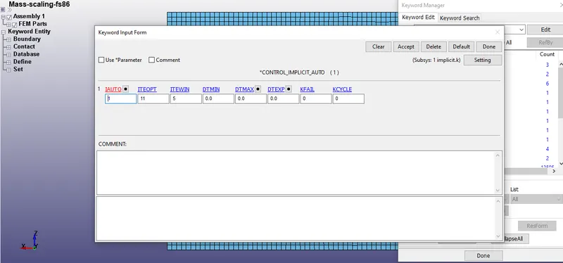
Fig, represents the assignment of ITEOPT and ITEWIN in the *control_implicit_Auto

• After that, in the control time step, a DT2MS value (3.5e-5) is assigned and the problem is solved by using the LS Run.

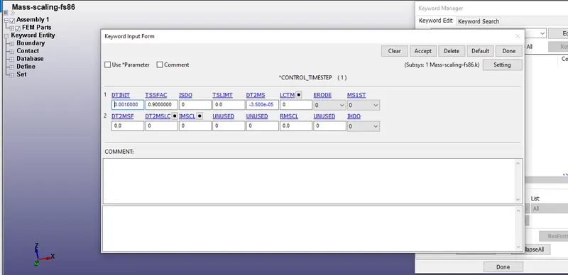
Fig, represents the assignment of DT2MS, value to the control time step

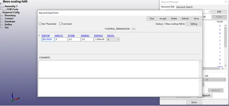
Fig, represents the end time given in the control_Termination card

• The end time of 600 seconds is given in the control termination card for both implicit and explicit analysis.
• After, that the implicit problem is solved by using LS-RUN.

OUTPUT RESULTS

HISTOGRAM OF MASS SCALING TRIALS WITH VARIOUS RUN TIME (FOR EXPLICIT ANALYSIS)

• The mass scaling trials are done by varying DT2MS values and the various DT2MS values and their corresponding run time values are noted. The histogram is plotted against Estimated time vs DT2MS.

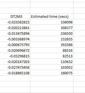
Fig, represents the varying DT2MS and their corresponding DT2MS values

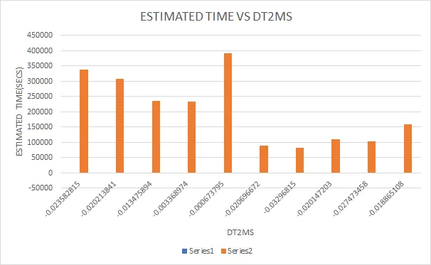
Fig, represents the histogram containing estimated time with DT2MS values.

• From, the histogram it is seen that for the DT2MS value of -0.1*10^-5 (-0.000673), the run time was found to be 392586 secs. From, the histogram it is evident that the increasing value of DT2MS has a lesser run-time when compared to those which have a decreasing value of DT2MS.
• From, the histogram it is noted that the lowest run time is found to be 82513(secs), and their corresponding DT2MS value is found to be (-0.03296).
• From, the histogram is found to be the DT2MS values with the exponential (e^-5) has a higher run time when compared to the exponential (e^-4).
• From, the histogram it is noted that for the DT2MS value of -1.03*e^-4 (-0.01886), the run time was found to be 160075 secs, this is the DT2MS value where the percentage increase of mass 8% is achieved for the model.

ADDITIONAL ANALYSIS ON EXPLICIT ANALYSIS (BY varying tssfac values)

• The explicit analysis is done additionally, by varying the tssfac values and by keeping the constant DT2MS values.
• DT2MS=1.03E^-4 , tssfac =0.9,0.8,0.7,0.6 ( the tssfac is varied from 0.9 to 0.6)

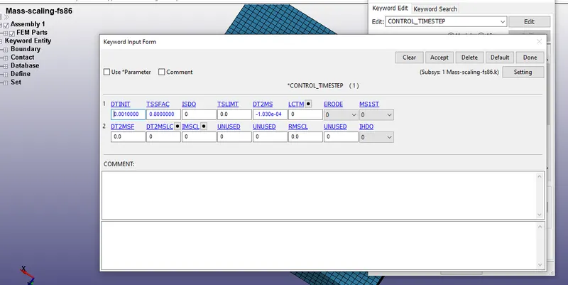
Fig, represents the varying tssfac with the constant DT2MS value

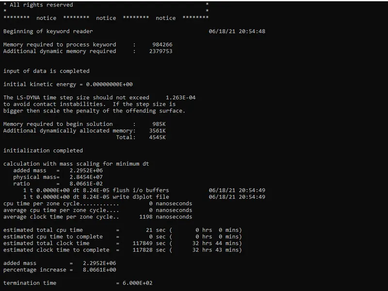
Fig, represents the normal termination of the explicit problem by varying tssfac to 0.8

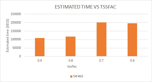
Fig, represents the estimated time vs tssfac values

• From, the figure it is understood that varying the tssfsac decreases the time step of the model and increases the run time of the model.
• From, the figure it is evident that by decreasing the tssfac value from 0.9 to 0.6, the run time of the model keeps on increasing, which means lower the Issac value it takes longer time to solve the model.
• Also, it is evident that for the tssfac value of 0.7, it took 200499 seconds approximately to run the model.
• Basically, the tssfac lowers the time step which inturn increases the time for solving the model.

• OUTPUT RESULTS FOR IMPLICIT ANALYSIS

CASE 1 (DT = 0.001)

• When the implicit analysis is done for the DT (0.001), with the ITEOPT of 11 and ITEWIN of 5, with the end time of 600 seconds, it took 5 hrs to solve 11,000 steps for solving 2% of the problem. It will take an additional 250 hours to complete the entire problem which is almost 60,000 steps.

ADDITIONAL ANALYSIS

CASE 2 (DT =0.01)

• when the DT value is increased to 0.1 for the same ITEOPT and ITEWIN, it took only 2 hours, 20 minutes to solve 6000 steps.

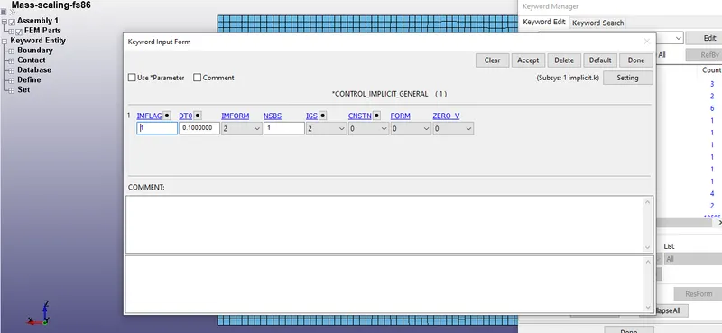
Fig, represents the DT value reduced to 0.1

Fig, represents the assignment of ITEOPT and ITEWIN to the control implicit auto

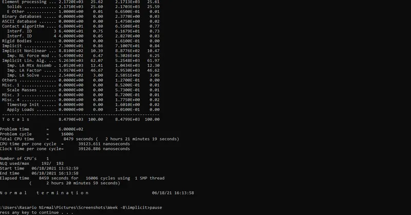
Fig, represents the normal termination of the implicit problem for the DT(0.1)

• From, the figure it is understood that for solving the implicit problem, it took 2 hours 20 minutes for solving the problem with the ITEOPT of 11 and ITEWIN of 5 and with the DT value of 0.1

CASE 3 (DT =0.1 , DTMIN=0.05 , DT=0.15)

• when the DT value is increased to 0.1 for the same ITEOPT and ITEWIN, but with assigning DTMIN = 0.05 & DTMAX=0.15, it took only 21 minutes and 58 seconds to solve the 6000 steps.

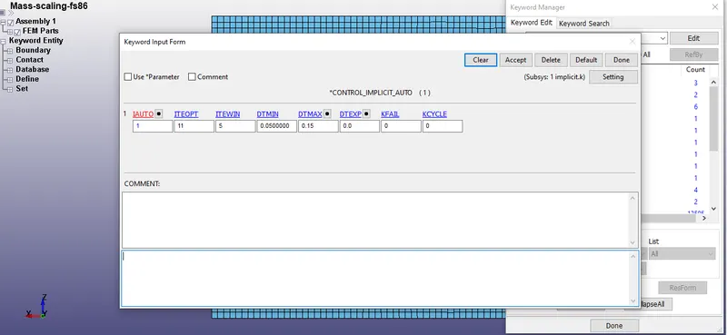
Fig, represents the assignment of DTMAX and DTMIN

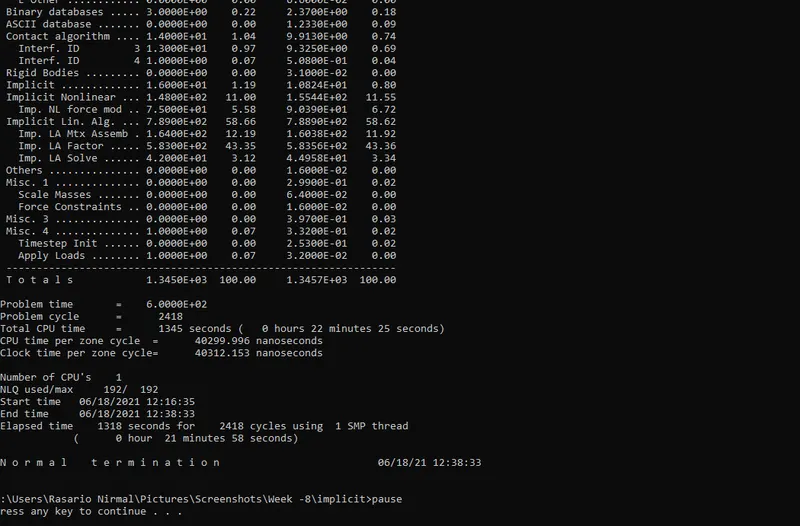
Fig, represents the normal termination of the implicit problem for CASE 3

• From, the figure it is understood that when the DTMAX and DTMIN are assigned, the LS DYNA solver optimized the iterations within the range of DTMAX and DTMIN and it only took 21 minutes and 58 seconds to solve the problem.

CONCLUSION

• Thus, the mass scaling is done for the model, and run time is reduced by mass scaling, and stability is attained.
• The trial and error methods are implemented to find the approximated DT2MS value, which contributed 8 % of mass to the model.
• The histograms are plotted and various run times and DT2MS values are compared successfully.
• An additional, analysis is conducted on the explicit analysis, how lowering the tssfac values affects the run time of the model by plotting a histogram.
• The implicit analysis is done successfully and their run-time is noted successfully.
• Additional analysis is done for case 2 and case 3, to evaluate how an increased DT(0.1), helps in reducing the run time of the model.