Week - 8 Mass Scaling

INTRODUCTION

One of the methods used in the industry to reduce the run time of an explicit FEM analysis is a technique called “Mass scaling”.

The run time of a FE simulation is mainly a function of the model size (the number of degrees of freedom) and the size of the solution step and the bigger the time step, faster the simulation.(not talking about the accuracy here).

I just want to emphasize that the time step size has a significant impact on the run time. As the size of the model is mostly not under our control, we have to play with “Time step” to reduce the runtime.

In other words, we have to increase the time step size. How we do this is effectively Mass Scaling.

As per the CFL (Courant-Friedrichs-Levy) condition, the stable time step for explicit analysis is

Here e_min is the size of the smallest mesh element.

c is the speed of the stress wave

The scaling factor is used for providing numerical stability.

The smallest element in the mesh has the biggest impact on the run time.

Let’s see what ‘c’ is made of.

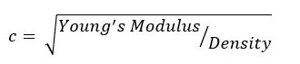
If we increase the density of the smallest element (add mass actually!), the time step size increases which is what we want.

And you have learnt the technique of mass scaling in a very simple rhetoric.

In other words, some amount of mass is added locally near the smallest elements in the mesh, which increases the density, thereby increasing the stable time step size henceforth reducing the solution run time.

PROCEDURE

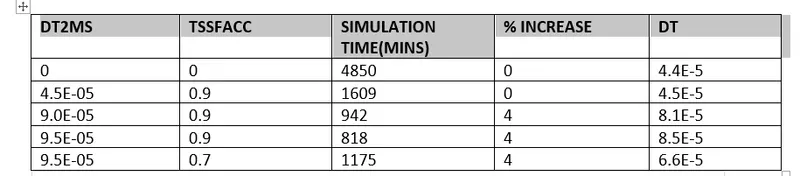
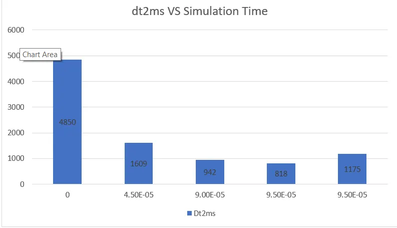
• In this project, the aim is to get a good understanding of the effect of mass scaling on explicit simulation by varying TSSFAC and DT2MS. The idea is to vary these values and see the differential results on a histogram.
• The effect of simulation time, percentage mass change and timestep change is recorded.
• An implicit simulation is run to see the difference in simulation characteristics.
• The file is opened in notepad++ and the values are edited.

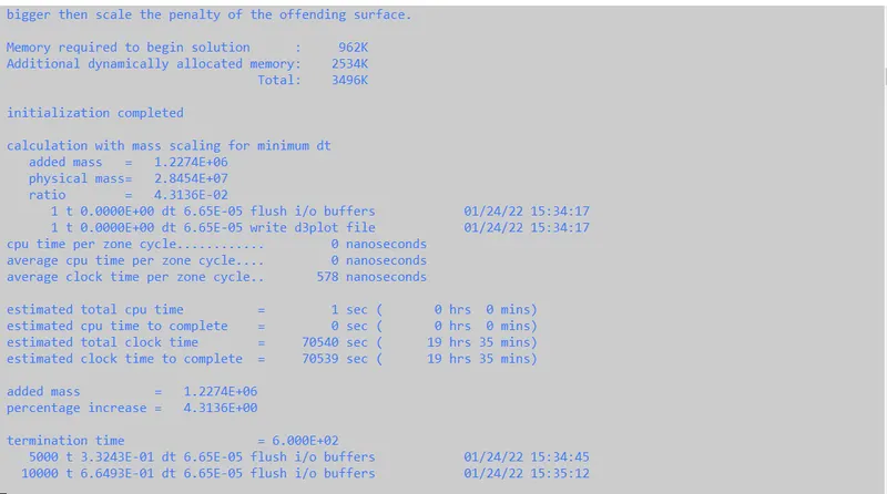
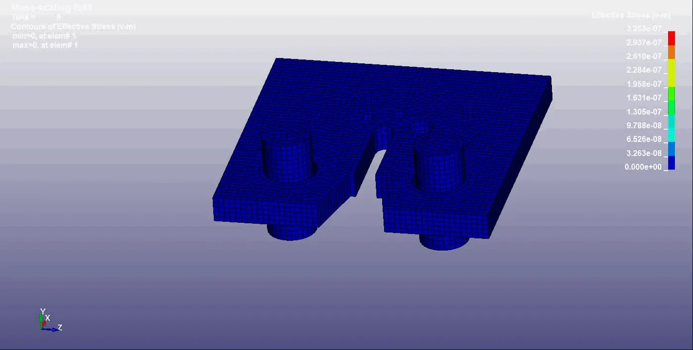
1. The specimen is imported into LS-Prepost and the the following values are set for the first run. DT2MS=0 ,TSSFACC=0 . It can be seen that the required simulation time is 80hrs:50mins, % mass increase of 0 and Dt of 4.4x10-5
2. The second run values are changed to DT2MS=-4.5x10-5 ,TSSFACC=0.9 . It can be seen that the required simulation time is 26hrs:49mins, % mass increase of 0 and Dt of 4.4x10-5
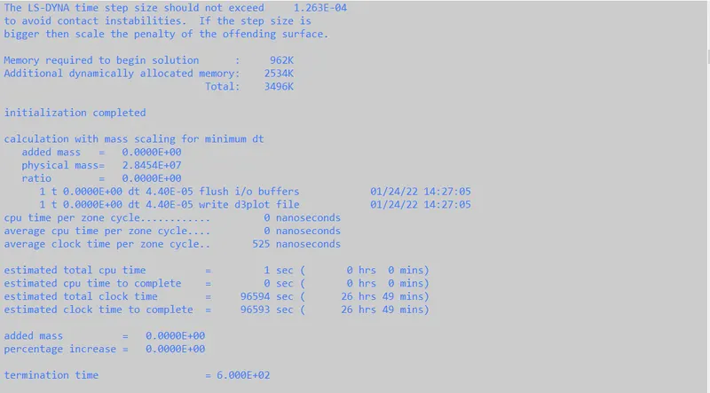
3. The third run values are changed to DT2MS=-9.0x10-5 ,TSSFACC=0.9 . It can be seen that the required simulation time is 15hrs:42mins, % mass increase of 2.7 and Dt of 8.1x10-5`
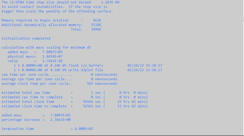
4. The fourth run values are changed to DT2MS=-9.5x10-5 ,TSSFACC=0.9 . It can be seen that the re6.65quired simulation time is 13hrs:42mins, % mass increase of 4 and Dt of 8.5x10-5
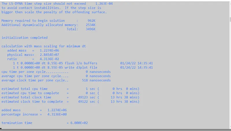
5. The fourth run values are changed to DT2MS=-9.5x10-5 ,TSSFACC=0.7 . It can be seen that the required simulation time is 19hrs:35mins, % mass increase of 4 and Dt of 6.65x10-5

IMPLICIT ANALYSIS

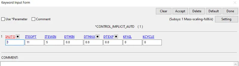
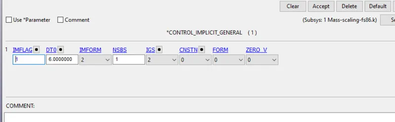
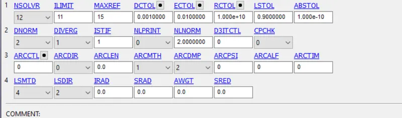
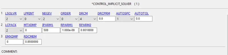
An implicit analysis is done to consider the differences in both approaches.

The folllowing control cards are created in Ls-Prepost below after the file is imported into the deck.

RESULTS

CONCLUSION

The results taken for the experiment describes exactly the effects of mass scaling with TSSFAC ,DT2MS etc.

From the above plotted histogram, it can clearly be seen that ,increasing of Dt2ms caused an increse in simulation time,% mass change and dt timestep.All this was seen with a constant TSSFACC of 0.9. When the TSSFACC was reduced , the was a drop in the dt timestep as the value has been scaled down compared to the 0.9 while keeping all other variables constant compared with the prior one. Mass of 4 percent was significantly added to the specimen when the Dt2ms was increased.

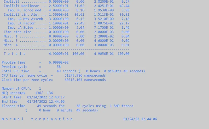
The explicit analysis was very short taking less than a minute to complete and the results were very good.Mass scaling isnt needed in implicit.

NB : files were to large to be attached so link for access is below

https://drive.google.com/drive/folders/1Wdkwq3spqoia0KfsbkwzyvSj2YFiXTEm?usp=sharing