Conjugate Heat Transfer simulation using Converge CFD

Aim:

• To setup conjugate heat transfer simulation of flow through a pipe using Converge CFD.

Objectives:

• To setup CHT simulation and confirm convergence through grid dependence test.
• To observe effect of change in supercycle stage interval.

A conjugate heat transfer simulation is a simulation where transfer of heat takes place through solids and fluids. In case of a fliud flowing through a pipe, the heat transfer occurs via conduction in the solid pipe and convection at the solid pipe-fluid interface surface. Since solving for heat transfer in solids and fluids takes place at different rates, supercycling had to be enabled. Supercycling helps speed up the solver for solid domain and hence it is commonly used in cases of conjugate heat transfer problems with a solid and liquid regions.

Geometry:

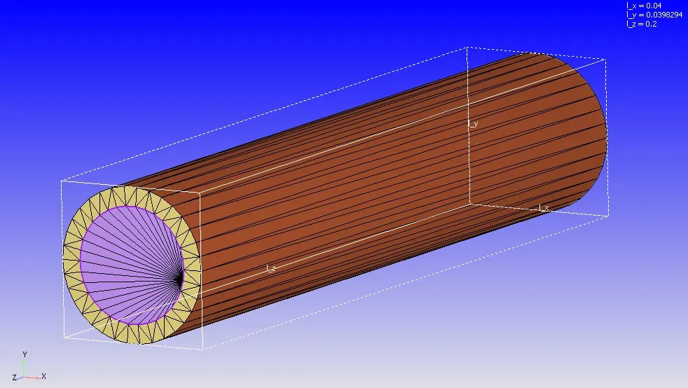
Fig.1 Geometry

The geometry is of a cylindrical pipe of length 0.2m, inner diameter 0.015 and thickness 0.05m.

Setup:

A transient simulation was set up with supercycle modelling enabled for the solid region. The material used for pipe was aluminium and fluid flowing through pipe was air. The Reynold's number for the flow needed to be set to 7000. Velocity for the same was found out by using the below formula;

Re = (rho*V*D)/(Dynamic viscosity)

Where, rho = density of fluid(Air) = 1.77 kg/m3

v = velocity of flow

D = inner diameter of the pipe = 0.015m

Dynamic viscosity(Air) = `1.846*10^-5`

Therefore; velocity, v= (Re*Dynamic viscosity)/(rho*D) = `(7000*1.846*10^-5)/(1.77*0.015)` = 4.9 m/s

• Boundary conditions:

1) Inflow boundary velocity = 4.9 m/s

2) Outflow boundary pressure = 101325 Pa

3) Outer walls- Slip boundary with heat flux 10000 W/m2

4) Interface:

Froward side- law of wall boundary

Reverse side - Slip boundary

• Regions:

Fluid region -Air(O2 & N2)

Solid region- Aluminium

• Turbulence modelling: RNG K-epsilon
• Supercycle modelling:

The supercycle stage interval was changed from 0.05s(baseline to 0.01s for observing its effect on the simulation.

• Base grid

For the grid dependence test, the following base grids were used(for dx,dy & dz);

1. 0.004m
2. 0.003m
3. 0.002m

For the remaining setup, default values were used.

Results & Observations:

The CHT simulation was run for 3 different grid sizes . The mesh generation and total number of cells for each case is shown below;

Grid Size(dx,dy,dz)	Total number of of cells
0.004 m	5000
0.003 m	10500
0.002 m	35600

Table.1 Grid sizes and cell count

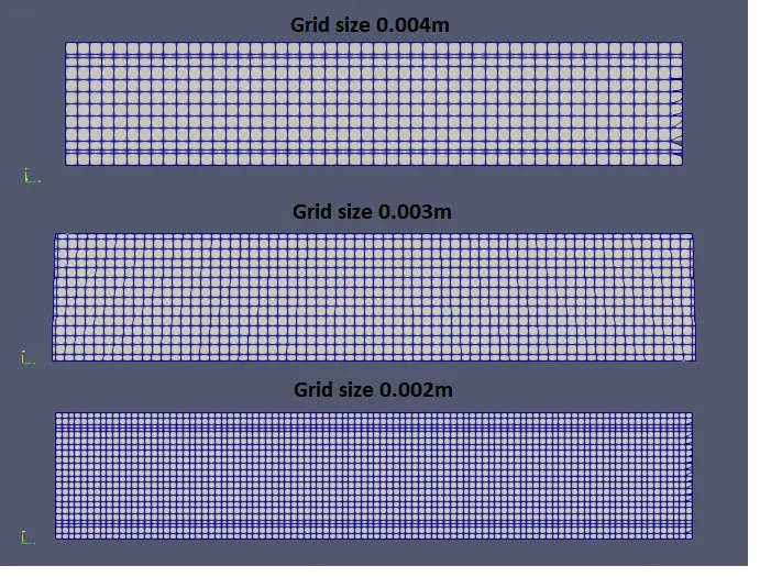
Fig.2 Mesh generation for different grid sizes

Grid Size(dx,dy,dz)	Max Yplus
0.004m	21
0.003m	22
0.002m	8.9

Table.2 Comparison of Max Yplus value for different grid sizes.

The simulation ran successfully for all three grid sizes. It was observed that for grid sizes of 0.004m and 0.003m, the Yplus value was in the transitioning range of laminar to turbulent which is undesired. But for the finer grid size of 0.002m, a max Yplus value of 8.9 was observed which is accepable as it is in laminar region.

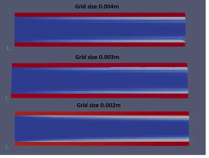
Fig.6 Final temperature contour

As expected, the final contour for the smallest grid size shows the temperature distribution with much clarity compared to the later two. It can be seen that the fluid is heated near the pipe surface by the time it reaches the outlet. The line plots for mean outlet temperature has been shown below.

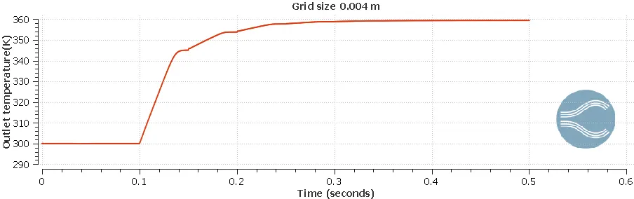
Plot.1 Mean oultet temperature(grid size 0.004m)

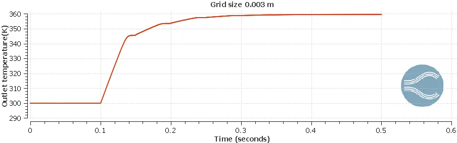
Plot.2 Mean oultet temperature(grid size 0.003m)

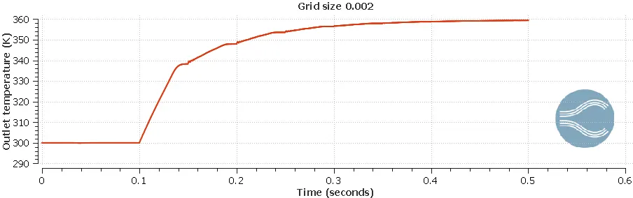
Plot.3 Mean oultet temperature(grid size 0.002m)

From analyzing the results for the three different grid sizes, the outlet mean temperature was found to be the same. From the grid dependency test, a mean outlet temperature of 360 K was observed. Hence, grid convergence had been acheived.

Simulation animation:

https://youtu.be/TgMLAOAeZQ0

The results obtained for simulation run with different supercycle stage intervals are discussed below.

supercyle stage interval(seconds)	Total simulation time (seconds)
0.03	579
0.02	559
0.01	500

Table.2 Supercycle stage interval and corresponding simulation run time.

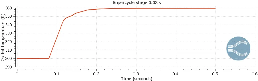
Plot.4 Mean outlet temperature(Supercycle stage interval 0.03s)

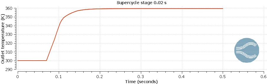
Plot.5 Mean outlet temperature(Supercycle stage interval 0.02s)

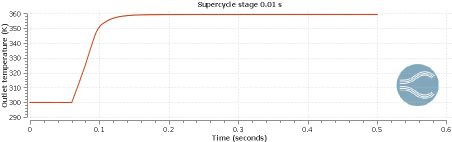
Plot.6 Mean outlet temperature(Supercycle stage interval 0.01s)

From running the simulation with three different supercycle stage intervals, although no notable changes where observed interms of final results, it was observed that the total simulation time was longer for a higher value of supercycle stage interval. Also, the outlet temperature converged quickly for a lower value of supercycle stage interval. A lower supercycle stage interval will solve for the solid region much quickly than a higher stage interval. Owing to this reason, the simulation time and convergence time shortened for a lower value of supercycle stage interval as observed.

Conclusion:

The Conjugate heat transfer simulation of flow of air through an aluminium pipe was carried out successfully. Grid dependence test was carried out by changing grid size from 0.004m to 0.003m and 0.002m in all three directions and observed its effects on outlet temperature and Yplus range. Observed the changes in output with changes in supercycle stage interval by reducing the interval from 0.05s to 0.01s.